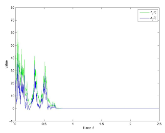
Figure 1.
States z_1(t) and z_2(t) of Example 5.1.


This work investigates the minimum eradication time in a controlled susceptible-infectious-recovered model with constant infection and recovery rates. The eradication time is defined as the earliest time the infectious population falls below a prescribed threshold and remains below it. Leveraging the fact that this problem reduces to solving a Hamilton-Jacobi-Bellman (HJB) equation, we propose a mesh-free framework based on a physics-informed neural network to approximate the solution. Moreover, leveraging the well-known structure of the optimal control of the problem, we efficiently obtain the optimal vaccination control from the minimum eradication time using the dynamic programming principle. To improve training stability and accuracy, we incorporate a variable scaling method and provide theoretical justification through a neural tangent kernel analysis. Numerical experiments show that this technique significantly enhances convergence, reducing the mean squared residual error by approximately 80% compared with standard physics-informed approaches. Furthermore, the method accurately identifies the optimal switching time. These results demonstrate the effectiveness of the proposed deep learning framework as a computational tool for solving optimal control problems in epidemic modeling as well as the corresponding HJB equations.
Citation: Minseok Kim, Yeongjong Kim, Yeoneung Kim. Physics-informed neural networks for optimal vaccination plan in SIR epidemic models[J]. Mathematical Biosciences and Engineering, 2025, 22(7): 1598-1633. doi: 10.3934/mbe.2025059
| [1] | Nina Huo, Bing Li, Yongkun Li . Global exponential stability and existence of almost periodic solutions in distribution for Clifford-valued stochastic high-order Hopfield neural networks with time-varying delays. AIMS Mathematics, 2022, 7(3): 3653-3679. doi: 10.3934/math.2022202 |
| [2] | Qinghua Zhou, Li Wan, Hongbo Fu, Qunjiao Zhang . Exponential stability of stochastic Hopfield neural network with mixed multiple delays. AIMS Mathematics, 2021, 6(4): 4142-4155. doi: 10.3934/math.2021245 |
| [3] | Li Wan, Qinghua Zhou, Hongbo Fu, Qunjiao Zhang . Exponential stability of Hopfield neural networks of neutral type with multiple time-varying delays. AIMS Mathematics, 2021, 6(8): 8030-8043. doi: 10.3934/math.2021466 |
| [4] | Ravi P. Agarwal, Snezhana Hristova . Stability of delay Hopfield neural networks with generalized proportional Riemann-Liouville fractional derivative. AIMS Mathematics, 2023, 8(11): 26801-26820. doi: 10.3934/math.20231372 |
| [5] | Yijia Zhang, Tao Xie, Yunlong Ma . Robustness analysis of exponential stability of Cohen-Grossberg neural network with neutral terms. AIMS Mathematics, 2025, 10(3): 4938-4954. doi: 10.3934/math.2025226 |
| [6] | Yuwei Cao, Bing Li . Existence and global exponential stability of compact almost automorphic solutions for Clifford-valued high-order Hopfield neutral neural networks with D operator. AIMS Mathematics, 2022, 7(4): 6182-6203. doi: 10.3934/math.2022344 |
| [7] | Tian Xu, Ailong Wu . Stabilization of nonlinear hybrid stochastic time-delay neural networks with Lévy noise using discrete-time feedback control. AIMS Mathematics, 2024, 9(10): 27080-27101. doi: 10.3934/math.20241317 |
| [8] | Zhigang Zhou, Li Wan, Qunjiao Zhang, Hongbo Fu, Huizhen Li, Qinghua Zhou . Exponential stability of periodic solution for stochastic neural networks involving multiple time-varying delays. AIMS Mathematics, 2024, 9(6): 14932-14948. doi: 10.3934/math.2024723 |
| [9] | Jin Gao, Lihua Dai . Anti-periodic synchronization of quaternion-valued high-order Hopfield neural networks with delays. AIMS Mathematics, 2022, 7(8): 14051-14075. doi: 10.3934/math.2022775 |
| [10] | Chantapish Zamart, Thongchai Botmart, Wajaree Weera, Prem Junsawang . Finite-time decentralized event-triggered feedback control for generalized neural networks with mixed interval time-varying delays and cyber-attacks. AIMS Mathematics, 2023, 8(9): 22274-22300. doi: 10.3934/math.20231136 |
This work investigates the minimum eradication time in a controlled susceptible-infectious-recovered model with constant infection and recovery rates. The eradication time is defined as the earliest time the infectious population falls below a prescribed threshold and remains below it. Leveraging the fact that this problem reduces to solving a Hamilton-Jacobi-Bellman (HJB) equation, we propose a mesh-free framework based on a physics-informed neural network to approximate the solution. Moreover, leveraging the well-known structure of the optimal control of the problem, we efficiently obtain the optimal vaccination control from the minimum eradication time using the dynamic programming principle. To improve training stability and accuracy, we incorporate a variable scaling method and provide theoretical justification through a neural tangent kernel analysis. Numerical experiments show that this technique significantly enhances convergence, reducing the mean squared residual error by approximately 80% compared with standard physics-informed approaches. Furthermore, the method accurately identifies the optimal switching time. These results demonstrate the effectiveness of the proposed deep learning framework as a computational tool for solving optimal control problems in epidemic modeling as well as the corresponding HJB equations.
Hopfield neural networks have recently sparked significant interest, due to their versatile applications in various domains including associative memory [1], image restoration [2], and pattern recognition [3]. In neural networks, time delays often arise due to the restricted switching speed of amplifiers [4]. Additionally, when examining long-term dynamic behavior, nonautonomous characteristics become apparent, with system coefficients evolving over time [5]. Moreover, in biological nervous systems, synaptic transmission introduces stochastic perturbations, adding an element of randomness [6]. As we know that time delays, nonautonomous behavior, and stochastic perturbations can induce oscillations and instability in neural networks. Hence, it becomes imperative to investigate the stability of stochastic delay Hopfield neural networks (SDHNNs) with variable coefficients.
The Lyapunov technique stands out as a powerful approach for examining the stability of SDHNNs. Wang et al. [7,8] and Chen et al. [9] employed the Lyapunov-Krasovskii functional to investigate the (global) asymptotic stability of SHNNs characterized by constant coefficients and bounded delay, respectively. Zhou and Wan [10] and Hu et al. [11] utilized the Lyapunov technique and some analysis techniques to investigate the stability of SHNNs with constant coefficients and bounded delay, respectively. Liu and Deng [12] used the vector Lyapunov function to investigate the stability of SHNNs with bounded variable coefficients and bounded delay. It is important to note that establishing a suitable Lyapunov function or functional can pose significant challenges, especially when dealing with infinite delay nonautonomous stochastic systems.
Meanwhile, the fixed point technique presents itself as another potent tool for stability analysis, offering the advantage of not necessitating the construction of a Lyapunov function or functional. Luo used this technique to consider the stability of several stochastic delay systems in earlier research [13,14,15]. More recently, Chen et al. [16] and Song et al. [17] explored the stability of SDNNs characterized by constant coefficients and bounded variable coefficients using the fixed point technique, yielding intriguing results. However, the fixed point technique has a limitation in the stability analysis of stochastic systems, stemming from the inappropriate application of the Hölder inequality.
Furthermore, integral or differential inequalities are also powerful techniques for stability analysis. Hou et al. [18], and Zhao and Wu [19] used the differential inequalities to consider stability of NNs, Wan and Sun [20], Sun and Cao [21], as well as Li and Deng [22] harnessed variation parameters and integral inequalities to explore the exponential stability of various SDHNNs with constant coefficients. In a similar vein, Ruan et al. [23] and Zhang et al. [24] utilized integral and differential inequalities to probe the pth moment exponential stability of SDHNNs characterized by bounded variable coefficients.
It is worth highlighting that the literature mentioned previously exclusively focused on investigating the exponential stability of SDHNNs, without addressing other decay modes. Generalized exponential stability was introduced in [25] for cellular neural networks without stochastic perturbations, and is a more general concept of stability which contains the usual exponential stability, polynomial stability, and logarithmical stability. It provides some new insights into the stability of dynamic systems. Motivated by the above discussion, we are prompted to explore the pth moment generalized exponential stability of SHNNs characterized by variable coefficients and infinite delay.
| {dzi(t)=[−ci(t)zi(t)+n∑j=1aij(t)fj(zj(t))+n∑j=1bij(t)gj(zj(t−δij(t)))]dt+n∑j=1σij(t,zj(t),zj(t−δij(t)))dwj(t),t≥t0,zi(t)=ϕi(t),t≤t0,i=1,2,...,n. | (1.1) |
It is important to note that the models presented in [20,21,25,26,27,28] are specific instances of system (1.1). System (1.1) incorporates several complex factors, including unbounded time-varying coefficients and infinite delay functions. As a result, discussing the stability and its decay rate for (1.1) becomes more complicated and challenging.
The contributions of this paper can be summarized as follows: (ⅰ) A new concept of stability is utilized for SDHNNs, namely the generalized exponential stability in pth moment. (ⅱ) We establish a set of multidimensional integral inequalities that encompass unbounded variable coefficients and infinite delay, which extends the works in [23]. (ⅲ) Leveraging these derived inequalities, we delve into the pth moment generalized exponential stability of SDHNNs with variable coefficients, and the work in [10,11,20,21,26,27] are improved and extended.
The structure of the paper is as follows: Section 2 covers preliminaries and provides a model description. In Section 3, we present the primary inequalities along with their corresponding proofs. Section 4 is dedicated to the application of these derived inequalities in assessing the pth moment generalized exponential stability of SDHNNs with variable coefficients. In Section 5, we present three simulation examples that effectively illustrate the practical applicability of the main results. Finally, Section 6 concludes our paper.
Let Nn={1,2,...,n}. |⋅| is the norm of Rn. For any sets A and B, A−B:={x|x∈A, x∉B}. For two matrixes C,D∈Rn×m, C≥D, C≤D, and C<D mean that every pair of corresponding parameters of C and D satisfy inequalities ≥, ≤, and <, respectively. ET and E−1 represent the transpose and inverse of the matrix E, respectively. The space of bounded continuous Rn-valued functions is denoted by BC:=BC((−∞,t0];Rn), for φ∈BC, and its norm is given by
| ‖φ‖∞=supθ∈(−∞,t0]|φ(θ)|<∞. |
(Ω,F,{Ft}t≥t0,P) stands for the complete probability space with a right continuous normal filtration {Ft}t≥t0 and Ft0 contains all P-null sets. For p>0, let LpFt((−∞,t0];Rn):=LpFt be the space of {Ft}-measurable stochastic processes ϕ={ϕ(θ):θ∈(−∞,t0]} which take value in BC satisfying
| ‖ϕ‖pLp=supθ∈(−∞,t0]E|ϕ(θ)|p<∞, |
where E represents the expectation operator.
In system (1.1), zi(t) represents the ith neural state at time t; ci(t) is the self-feedback connection weight at time t; aij(t) and bij(t) denote the connection weight at time t of the jth unit on the ith unit; fj and gj represent the activation functions; σij(t,zj(t),zj(t−δij(t))) stands for the stochastic effect, and δij(t)≥0 denotes the delay function. Moreover, {ωj(t)}j∈Nn is a set of Wiener processes mutually independent on the space (Ω,F,{Ft}t≥0,P); zi(t,ϕ) (i∈Nn) represents the solution of (1.1) with an initial condition ϕ=(ϕ1,ϕ2,...,ϕn)∈LpFt, sometimes written as zi(t) for short. Now, we introduce the definition of generalized exponentially stable in pth (p≥2) moment.
Definition 2.1. System (1.1) is pth (p≥2) moment generalized exponentially stable, if for any ϕ∈LpFt, there are κ>0 and c(u)≥0 such that limt→+∞∫tt0c(u)du→+∞ and
| E|zi(t,ϕ)|p≤κmaxj∈Nn{‖ϕj‖pLp}e−∫tt0c(u)du,i∈Nn,t≥t0, |
where −∫tt0c(u)du is the general decay rate.
Remark 2.1. Lu et al. [25] proposed the generalized exponential stability for neural networks without stochastic perturbations, we extend it to the SDHNNs.
Remark 2.2. We replace ∫tt0c(u)du by λ(t−t0), λln(t−t0+1), and λln(ln(t−t0+e)) (λ>0), respectively. Then (1.1) is exponentially, polynomially, and logarithmically stable in pth moment, respectively.
Lemma 2.1. [29] For a square matrix Λ≥0, if ρ(Λ)<1, then (I−Λ)−1≥0, where ρ(⋅) is the spectral radius, and I and 0 are the identity and zero matrices, respectively.
Consider the following inequalities
| {yi(t)≤ψi(0)e−∫tt0γi(u)du+n∑j=1αij∫tt0e−∫tsγi(u)duγi(s)sups−ηij(s)≤v≤syj(v)ds,t≥t0,yi(t)=ψi(t)∈BC,t∈(−∞,t0],i∈Nn, | (3.1) |
where yi(t), γi(t), and ηij(t) are non-negative functions and αij≥0, i,j∈Nn.
Lemma 3.1. Regrading system (3.1), let the following hypotheses hold:
(H.1) For i,j∈Nn, there exist γ(t) and γi>0 such that
| 0≤γiγ(t)≤γi(t)fort≥t0,limt→+∞∫tt0γ(u)du→+∞,supt≥t0{∫tt−ηij(t)γ∗(u)du}:=ηij<+∞, |
where γ∗(t)=γ(t), for t≥t0, and γ∗(t)=0, for t<t0.
(H.2) ρ(α)<1, where α=(αij)n×n.
Then, there is a κ>0 such that
| yi(t)≤κmaxj∈Nn{‖ψj‖∞}e−λ∫tt0γ(u)du,i∈Nn,t≥t0. |
Proof. For t≥t0, multiply eλ∫tt0γ(u)du on both sides of (3.1), and one has
| eλ∫tt0γ(u)duyi(t)≤ψi(t0)eλ∫tt0γ(u)due−∫tt0γi(u)du+n∑j=1eλ∫tt0γ(s)dsαij∫tt0e−∫tsγi(u)duγi(s)sups−ηij(s)≤v≤syj(v)ds:=Ii1(t)+Ii2(t),i∈Nn, | (3.2) |
where λ∈(0,mini∈Nn{γi}) is a sufficiently small constant which will be explained later. Define
| Hi(t):=supξ≤t{eλ∫ξt0γ∗(u)duyi(ξ)}, |
i∈Nn and t≥t0. Obviously,
| Ii1(t)=ψi(t0)eλ∫tt0γ(u)due−∫tt0γi(u)du≤e(λ−γi)∫tt0γ(u)duψi(t0)≤ψi(t0),i∈Nn,t≥t0. | (3.3) |
Further, it follows from (H.1) that
| Ii2(t)≤n∑j=1αij∫tt0e−∫tsγi(u)duγi(s)eλ∫ss−ηij(s)γ∗(u)dusups−ηij(s)≤v≤s{yj(v)}eλ∫s−ηij(s)t0γ∗(u)dueλ∫tsγ(u)duds≤n∑j=1αijeληij∫tt0e−∫ts(γi(u)−λγ(u))duγi(s)sups−ηij(s)≤v≤s{yj(v)eλ∫vt0γ∗(u)du}ds≤n∑j=1αijeληijHj(t)∫tt0e−∫ts(γi(u)−λγ(u))duγi(s)ds≤n∑j=1αijeληijHj(t)∫tt0e−∫ts(γi(u)−λγiγi(u))duγi(s)ds≤γiγi−λn∑j=1αijeληijHj(t),i∈Nn,t≥t0. | (3.4) |
By (3.2)–(3.4), we have
| eλ∫tt0γ(s)dsyi(t)≤ψi(t0)+γiγi−λn∑j=1αijeληijHj(t),i∈Nn,t≥t0. |
By the definition of Hi(t), we get
| Hi(t)≤ψi(t0)+γiγi−λn∑j=1αijeληijHj(t),i∈Nn,t≥t0, |
i.e.,
| H(t)≤ψ(t0)+ΓαeληH(t)Γ−λI,t≥t0, | (3.5) |
where H(t)=(H1(t),...,Hn(t))T, ψ(t0)=(ψ1(t0),...,ψn(t0))T, Γ=diag(γ1,...,γn), and αeλη=(αijeληij)n×n. Since ρ(α)<1 and α≥0, then there is a small enough λ>0 such that
| ρ(ΓαeληΓ−λI)<1 and ΓαeληΓ−λI≥0. |
From Lemma 2.1, we get
| (I−ΓαeληΓ−λI)−1≥0. |
Denote
| N(λ)=(I−ΓαeληΓ−λI)−1=(Nij(λ))n×n. |
From (3.5), we have
| H(t)≤N(λ)ψ(t0),t≥t0. |
Therefore, for i∈Nn, we get
| yi(t)≤n∑i=1Nij(λ)ψi(t0)e−λ∫tt0γ(u)du≤n∑j=1Nij(λ)‖ψj‖∞e−λ∫tt0γ(u)du,t≥t0, |
and then there exists a κ>0 such that
| yi(t)≤κmaxi∈Nn{‖ψi‖∞}e−λ∫tt0γ(u)du,i∈Nn,t≥t0. |
This completes the proof.
Consider the following differential inequalities
| {D+yi(t)≤−γi(t)yi(t)+n∑j=1αijγi(t)supt−ηij(t)≤s≤tyj(s),t≥t0,yi(t)=ψi(t)∈BC,t∈(−∞,t0],i∈Nn, | (3.6) |
where D+ is the Dini-derivative, yi(t), γi(t), and ηij(t) are non-negative functions, and αij≥0, i,j∈Nn.
Lemma 3.2. For system (3.6), under hypotheses (H.1) and (H.2), there are κ>0 and λ>0 such that
| yi(t)≤κmaxi∈Nn{‖ψi‖∞}e−λ∫tt0γ(u)du,i∈Nn,t≥t0. |
Proof. For t>t0, multiply e∫tt0γi(u)du (i∈Nn) on both sides of (3.6) and perform the integration from t0 to t. We have
| yi(t)≤ψi(0)e−∫tt0γi(u)du+n∑j=1∫tt0e−∫tsγi(u)duαijγi(s)sups−ηij(s)≤v≤syj(v)ds,i∈Nn. |
The proof is deduced from Lemma 3.1.
Remark 3.1. For a given matrix M=(mij)n×n, we have ρ(M)≤‖M‖, where ‖⋅‖ is an arbitrary norm, and then we can obtain some conditions for generalized exponential stability. In addition, for any nonsingular matrix S, define the responding norm by ‖M‖S=‖S−1MS‖. Let S=diag{ξ1,ξ2,...,ξn}, then for the row, column, and the Frobenius norm, the following conditions imply ‖M‖S<1:
(1) n∑j=1(ξiξj|mij|)<1 for i∈Nn;
(2) n∑i=1(ξiξj|mij|)<1 for i∈Nn;
(3) n∑i=1n∑j=1(ξiξj|mij|)2<1.
Remark 3.2. Ruan et al. [23] investigated the special case of inequalities (3.6), i.e., γi(t)=γi and ηij(t)=ηij. They obtained that system (3.6) is exponentially stable provided
| γi>n∑j=1αij,i∈Nn. | (3.7) |
From Remark 3.1, we know condition ρ(α)<1 (α=(αijγi)n×n) is weaker than (3.7). Moreover, we discuss the generalized exponential stability which contains the normal exponential stability. This means that our result improves and extends the result in [23].
This section considers the pth moment generalized exponential stability of (1.1) by applying Lemma 3.1. To obtain the pth moment generalized exponential stability, we need the following conditions.
(C.1) For i,j∈Nn, there are c(t) and ci>0 such that
| 0≤cic(t)≤ci(t) for t≥t0,limt→+∞∫tt0c(s)ds→+∞,supt≥t0{∫tt−δij(t)c∗(s)ds}:=δij<+∞, |
where c∗(t)=c(t), for t≥t0, and c(t)=0, for t<t0.
(C.2) The mappings fj and gj satisfy fj(0)=gj(0)=0 and the Lipchitz condition with Lipchitz constants Fj>0 and Gj>0 such that
| |fj(v1)−fj(v2)|≤Fj|v1−v2|,|gj(v1)−gj(v2)|≤Gj|v1−v2|,j∈Nn,∀v1,v2∈R. |
(C.3) The mapping σij satisfies σij(t,0,0)≡0 and ∀u1,u2,v1,v2∈R, and there are μij(t)≥0 and νij(t)≥0 such that
| |σij(t,u1,v1)−σij(t,u2,v2)|2≤μij(t)|u1−u2|2+νij(t)|v1−v2|2,i,j∈Nn,t≥t0. |
(C.4) For i,j∈Nn,
| sup{t|t≥t0}−{t|ci(t)=|aij(t)|Fj+|bij(t)|Gj=0}{|aij(t)|Fj+|bij(t)|Gjci(t)}:=ρ(1)ij,sup{t|t≥t0}−{t|ci(t)=μij(t)+νij(t)}{μij(t)+νij(t)ci(t)}:=ρ(2)ij. |
(C.5)
| ρ(M+Ω(1)p+(p−1)Ω(2)p)<1, |
where M=diag(m1,m2,...,mn), mi=(p−1)n∑j=1ρ(1)ijp+(p−1)(p−2)n∑j=1ρ(2)ij2p, Ω(k)=(ρ(k)ij)n×n, k∈N2, and p≥2.
Conditions (C.1)–(C.4) guarantee the existence and uniqueness of (1.1) [30].
Theorem 4.1. Under conditions (C.1)–(C.5), system (1.1) is pth moment generalized exponentially stable with decay rate −λ∫tt0c(s)ds, λ>0.
Proof. By the Itô formula, one can obtain
| dzpi(t)=[−pci(t)zpi(t)+n∑j=1paij(t)fj(zj(t))zp−1i(t)+n∑j=1pbij(t)gj(zj(t−δij(t)))zp−1i(t)+n∑j=1p(p−1)2|σij(t,zj(t),zj(t−δij(t)))|2zp−2i(t)]dt+n∑j=1pσij(t,zj(t),zj(t−δij(t)))zp−1i(t)dwj(t),i∈Nn,t≥t0. |
So we get
| zpi(t)=ϕpi(t0)+∫tt0[−pci(s)zpi(s)+n∑j=1paij(s)fj(zj(s))zp−1i(s)+n∑j=1pbij(s)gj(zj(s−δij(s)))zp−1i(s)+n∑j=1p(p−1)2|σij(s,zj(s),zj(s−δij(s)))|2zp−2i(s)]ds+n∑j=1∫tt0pσij(s,zj(s),zj(s−δij(s)))zp−1i(s)dwj(s),i∈Nn,t≥t0. |
Since E[∫tt0pσij(s,zj(s),zj(s−δij(s)))zp−1i(s)dwj(s)]=0 for i∈Nn and t≥t0, we have
| E[zpi(t)]=E[ϕpi(t0)]+∫tt0E[−pci(s)zpi(s)+n∑j=1paij(s)fj(zj(s))zp−1i(s)+n∑j=1pbij(s)gj(zj(s−δij(s)))zp−1i(s)+n∑j=1|σij(s,zj(s),zj(t−δij(s)))|2p(p−1)2zp−2i(s)]ds,i∈Nn,t≥t0, |
i.e.,
| dE[zpi(t)]=−pci(t)E[zpi(t)]dt+E[n∑j=1paij(t)fj(zj(t))zp−1i(t)+n∑j=1pbij(t)gj(zj(t−δij(t)))zp−1i(t)+n∑j=1p(p−1)2|σij(t,zj(t),zj(t−δij(t)))|2zp−2i(t)]dt,i∈Nn,t≥t0. |
For i∈Nn and t≥t0, using the variation parameter approach, we get
| E[zpi(t)]=E[ϕpi(t0)]e−∫tt0pci(s)ds+∫tt0e−∫tspci(u)duE[n∑j=1paij(s)fj(zj(s))zp−1i(s)+n∑j=1pbij(s)gj(zj(s−δij(s)))zp−1i(s)+n∑j=1p(p−1)2|σij(s,zj(s),zj(s−δij(s)))|2zp−2i(s)]ds. |
For i∈Nn and t≥t0, conditions (C.2)–(C.4) and the Young inequality yield
| E|zi(t)|p≤E|ϕi(t0)|pe−∫tt0pci(u)du+n∑j=1∫tt0e−∫tspci(u)dup|aij(s)|FjE|zj(s)zp−1i(s)|ds+n∑j=1∫tt0e−∫tspci(u)dup|bij(s)|GjE|zj(s−δij(s))zp−1i(s)|ds+n∑j=1∫tt0e−∫tspci(u)dup(p−1)2μij(s)E|z2j(s)zp−2i(s)|ds+n∑j=1∫tt0e−∫tspci(u)dup(p−1)2νij(s)E|z2j(s−δij(s))zp−2i(s)|ds≤E|ϕi(t0)|pe−∫tt0pci(u)du+n∑j=1∫tt0e−∫tspci(u)du|aij(s)|Fj(E|zj(s)|p+(p−1)E|zi(s)|p)ds+n∑j=1∫tt0e−∫tspci(u)du|bij(s)|Gj(E|zj(s−δij(s))|p+(p−1)E|zi(s)|p)ds+n∑j=1∫tt0e−∫tspci(u)duμij(s)((p−1)E|zj(s)|p+(p−1)(p−2)2E|zi(s)|p)ds+n∑j=1∫tt0e−∫tspci(u)duνij(s)((p−1)E|zj(s−δij(s))|p+(p−1)(p−2)2E|zi(s)|p)ds≤E|ϕi(t0)|pe−∫tt0pci(u)du+n∑j=1∫tt0e−∫tspci(u)du(ρ(1)ij+(p−1)ρ(2)ij)ci(s)sups−δij(s)≤v≤sE|zj(v)|pds+n∑j=1∫tt0e−∫tspci(u)du((p−1)ρ(1)ij+(p−1)(p−2)2ρ(2)ij)ci(s)sups−δij(s)≤v≤sE|zi(v)|pds. |
Then, all of the hypotheses of Lemma 3.1 are satisfied. So there exists κ>0 and λ>0 such that
| E|zi(t)|p≤κmaxj∈Nn{‖ϕj‖pLp}e−λ∫tt0c(u)du,i∈Nn,t≥t0. |
This completes the proof.
Remark 4.1. Huang et al.[27] and Sun and Cao [21] considered the special case of (1.1), i.e., aij(t)≡aij, bij(t)≡bij, ci(t)≡ci, μij(t)≡μj, νij(t)≡νj, and δij(t)≡δj(t) is a bounded delay function. [27] showed that system (1.1) is pth moment exponentially stable provided that there are positive constants ξi,...,ξn such that N1>N2>0, where
| N1=mini∈Nn{pci−n∑j=1(p−1)|aij|(Fj+Gj)+n∑j=1ξjξi(|aji|Fi+(p−1)μi)+n∑j=1(p−1)(p−2)2(μi+νi)} |
and
| N2=maxi∈Nn{n∑j=1ξjξi(|bji|Gi+(p−1)νi)}. |
The above conditions imply that for each i∈Nn,
| pci−n∑j=1(p−1)|aij|(Fj+Gj)+n∑j=1ξjξi(|aji|Fi+|bji|Gi+(p−1)(μi+νj))+n∑j=1(p−1)(p−2)2(μi+νi)>0. |
Then
| 0≤n∑j=1(p−1)|aij|(Fj+Gj)pci+n∑j=1ξjξi(|aji|Fi+|bji|Gi+(p−1)(μi+νj)pci)+n∑j=1(p−1)(p−2)2pci(μi+νi)<1. | (4.1) |
From Remark 3.1, we know condition (4.1) implies
| ρ(M+Ω(1)p+(p−1)Ω(2)p)<1, |
and this means that this paper improves and enhances the results in [27]. Similarly, our results also improve and enhance the results in [10,11,26]. Besides, the results in [21] required the following conditions to guarantee the pth moment exponential stability, i.e.,
| ρ(C−1(M∗M1I+M∗M2I+NN1+NN2))<1, |
where
| C=diag(c1,c2,...,cn),M∗=diag((4c1)p−1,(4c2)p−1,...,(4cn)p−1), |
| N1=(dij)n×n,dij=μp/2j,N2=(eij)n×n,eij=νp/2j, |
| M1=diag((n∑j=1|a1jFj|pp−1)p−1,(n∑j=1|a2jFj|pp−1)p−1,...,(n∑j=1|anjFj|pp−1)p−1), |
| M2=diag((n∑j=1|b1jGj|pp−1)p−1,(n∑j=1|b2jGj|pp−1)p−1,...,(n∑j=1|bnjGj|pp−1)p−1), |
| N=diag(4p−1Cpnp−1c1−p/21,4p−1Cpnp−1c1−p/22,...,4p−1Cpnp−1c1−p/2n)(Cp≥1). |
From the matrix spectral analysis [29], we can get
| ρ(M+Ω(1)p+(p−1)Ω(2)p)<ρ(C−1(M∗M1I+M∗M2I+NN1+NN2). |
The above discussion shows that our results improve and extend the works in [21]. Similarly, our results also improve and broaden the results in [20].
Remark 4.2. When c_i(t)\equiv c_i , a_{ij}(t)\equiv a_{ij} , b_{ij}(t)\equiv b_{ij} , \delta_{ij}(t)\equiv\delta_{j} , and \sigma_{ij}(t, z_j(t), z_j(t-\delta_{ij}(t)))\equiv0 , then (1.1) turns to be the following HNNs
| \begin{equation} dz_i(t) = \bigg[-c_iz_i(t)+\sum\limits_{j = 1}^na_{ij}f_j(z_j(t))+\sum\limits_{j = 1}^nb_{ij}g_j(z_j(t-\delta_{j}))\bigg]dt,\quad i\in \mathbb{N}_n,\quad t\geq t_0, \end{equation} | (4.2) |
or
| \begin{equation} dz(t) = \bigg[-Cz(t)+Af(z(t))+Bg(z_{\delta}(t))\bigg]dt,\quad t\geq t_0,\\ \end{equation} | (4.3) |
where z(t) = (z_1(t), ..., z_n(t))^T , C = diag(c_1, ..., c_n) > 0 , A = (a_{ij})_{n\times n} , B = (b_{ij})_{n\times n} , f(x(t)) = (f_1(z_1(t)), ..., f_n(z_n(t)))^T , and g(z_{\delta}(t)) = (g_1(z_1(t-\delta_1)), ..., g_n(z_n(t-\delta_n)))^T . This model was discussed in [16,28]. For (4.3), using our approach can get the subsequent corollary.
Corollary 4.1. Under condition (\mathbf{C.2}) , if \rho(C^{-1}D) < 1 , then (4.3) is exponentially stable, where D = (|a_{ij}F_j|+|b_{ij}G_j|)_{n\times n} .
Note that Lai and Zhang [28] (Theorem 4.1) and Chen et al. [16] (Corollary 5.2) required the following conditions
| \begin{equation*} \max\limits_{i\in\mathbb{N}_n}\bigg[\frac{1}{c_i}\sum\limits_{j = 1}^n|a_{ij}F_j|+\frac{1}{c_i}\sum\limits_{j = 1}^n|b_{ij}G_j|\bigg] < \frac{1}{\sqrt{n}} \end{equation*} |
and
| \begin{equation*} \sum\limits_{j = 1}^n\frac{1}{c_i}\max\limits_{i\in\mathbb{N}_n}|a_{ij}F_j|+\sum\limits_{j = 1}^n\frac{1}{c_i}\max\limits_{i\in\mathbb{N}_n}|b_{ij}G_j| < 1 \end{equation*} |
to ensure the exponential stability, respectively. From Remark 3.1, we know that Corollary 4.1 is weaker than Theorem 4.1 in [28] and Corollary 5.2 in [16]. This improves and extends the results in [16,28].
Now, we give three examples to illustrate the effectiveness of the main result.
Example 5.1. Consider the following SDHNNs:
| \begin{eqnarray} \left\{ \begin{array}{ll}dz_i(t) = \bigg[-c_i(t)z_i(t)+\sum^{2}\limits_{j = 1}a_{ij}(t)f_j(z_j(t))+\sum^{2}\limits_{j = 1}b_{ij}(t)g_j(z_j(0.5t))\bigg]dt\\ \quad\quad\qquad+\sum^{2}\limits_{j = 1}\sigma_{ij}(t,z_j(t),z_j(0.5t))dw_j(t),\quad t\geq 0,\\ z_i(0) = \phi_i(0),\quad i\in\mathbb{N}_2, \end{array} \right. \end{eqnarray} | (5.1) |
where c_1(t) = 10(t+1) , c_2(t) = 20(t+2) , a_{11}(t) = b_{11}(t) = 0.5(t+1) , a_{12}(t) = b_{12}(t) = t+1 , a_{21}(t) = b_{21}(t) = 2(t+2) , a_{22}(t) = b_{22}(t) = 2.5(t+2) , f_1(u) = f_2(u) = arctanu , g_1(u) = g_2(u) = 0.5(|u+1|-|u-1|) , \sigma_{11}(t, u, v) = \frac{\sqrt{2(t+1)}(u-v)}{2} , \sigma_{12}(t, u, v) = 2\sqrt{(t+1)}(u-v) , \sigma_{21}(t, u, v) = \sqrt{(t+1)}(u-v) , \sigma_{22}(t, u, v) = \frac{\sqrt{10(t+2)}(u-v)}{2} , \delta_{11}(t) = \delta_{21}(t) = \delta_{12}(t) = \delta_{22}(t) = 0.5t , and \phi(0) = (40, 20) .
Choose c(t) = \frac{1}{t+1} , and then \sup\limits_{t\geq0}\bigg\{\int^t_{0.5t}\frac{1}{s+1}ds\bigg\} = \ln2 . We can find F_1 = F_2 = G_1 = G_2 = 1 , \rho^{(1)}_{11} = 0.1 , \rho^{(1)}_{12} = 0.2 , \rho^{(1)}_{21} = 0.2 , \rho^{(1)}_{22} = 0.25 , \rho^{(2)}_{11} = 0.2 , \rho^{(2)}_{12} = 1.6 , \rho^{(2)}_{21} = 0.2 , and \rho^{(2)}_{22} = 0.5 . Then
| \begin{equation*} \rho{ \left( \begin{array}{ccc} \rho_{11}^{(1)}+0.5\rho_{12}^{(1)}+0.5\rho_{11}^{(2)} & 0.5\rho_{12}^{(1)}+0.5\rho_{12}^{(2)} \\ 0.5\rho_{21}^{(1)}+0.5\rho_{21}^{(2)}& \rho_{22}^{(1)}+0.5\rho_{21}^{(1)}+0.5\rho_{22}^{(2)} \end{array} \right )} = \rho{ \left( \begin{array}{ccc} 0.3 & 0.9 \\ 0.2& 0.6 \end{array} \right )} = 0.9 < 1. \end{equation*} |
Then (\mathbf{C.1}) – (\mathbf{C.5}) are satisfied (p = 2) . So (5.1) is generalized exponentially stable in mean square with a decay rate -\lambda\int^t_0\frac{1}{1+s}ds = -\lambda ln(1+t) , \lambda > 0 (see Figure 1).
Remark 5.1. It is noteworthy that all variable coefficients and delay functions in Example 5.1 are unbounded, and then the results in [12,23] are not applicable in this example.
Example 5.2. Consider the following SDHNNs:
| \begin{eqnarray} \left\{ \begin{array}{ll}dz_i(t) = \bigg[-c_i(t)z_i(t)+\sum\limits_{j = 1}^2a_{ij}(t)f_j(z_j(t))+\sum\limits_{j = 1}^2b_{ij}(t)g_j(z_j(t-\delta_{ij}(t)))\bigg]dt\\ \quad\quad\qquad+\sum\limits_{j = 1}^2\sigma_{ij}(t,z_j(t),z_j(t-\delta_{ij}(t)))dw_j(t),\quad\quad\quad\quad\quad\quad\quad\quad\quad t\geq 0,\\ z_i(t) = \phi_i(t),\quad t\in[-\pi,0],\quad i\in\mathbb{N}_2, \end{array} \right. \end{eqnarray} | (5.2) |
where c_1(t) = 20(1-sint) , c_2(t) = 10(1-sint) , a_{11}(t) = b_{11}(t) = 2(1-sint) , a_{12}(t) = b_{12}(t) = 4(1-sint) , a_{21}(t) = b_{21}(t) = 0.5(1-sint) , a_{22}(t) = b_{22}(t) = 1.5(1-sint) , f_1(u) = f_2(u) = arctanu , g_1(u) = g_2(u) = 0.5(|u+1|-|u-1|) , \sigma_{11}(t, u, v) = \sqrt{2(1-sint)}(u-v) , \sigma_{12}(t, u, v) = \sqrt{6(1-sint)}(u-v) , \sigma_{21}(t, u, v) = \frac{\sqrt{(1-sint)}(u-v)}{2} , \sigma_{22}(t, u, v) = \frac{\sqrt{(1-sint)}(u-v)}{2} , \delta_{11}(t) = \delta_{21}(t) = \delta_{12}(t) = \delta_{22}(t) = \pi|\cos t| , and \phi(t) = (40, 20) for t\in[-\pi, 0] .
Choose c(t) = 1-\sin t , and then \sup\limits_{t\geq0}\int^t_{t-\pi|\cos t|}\big(1-\sin s\big)^*ds = \pi+2 . We can find F_1 = F_2 = G_1 = G_2 = 1 , \rho^{(1)}_{11} = 0.2 , \rho^{(1)}_{12} = 0.4 , \rho^{(1)}_{21} = 0.1 , \rho^{(1)}_{22} = 0.3 , \rho^{(2)}_{11} = 0.4 , \rho^{(2)}_{12} = 1.2 , \rho^{(2)}_{21} = 0.1 , and \rho^{(2)}_{22} = 0.1 . Then
| \begin{equation*} \rho{ \left( \begin{array}{ccc} \rho_{11}^{(1)}+0.5\rho_{12}^{(1)}+0.5\rho_{11}^{(2)} & 0.5\rho_{12}^{(1)}+0.5\rho_{12}^{(2)} \\ 0.5\rho_{21}^{(1)}+0.5\rho_{21}^{(2)}& \rho_{22}^{(1)}+0.5\rho_{21}^{(1)}+0.5\rho_{22}^{(2)} \end{array} \right )} = \rho{ \left( \begin{array}{ccc} 0.6 & 0.8 \\ 0.1& 0.4 \end{array} \right )} = 0.8 < 1. \end{equation*} |
Then (\mathbf{C.1}) – (\mathbf{C.5}) are satisfied (p = 2) . So (5.2) is generalized exponentially stable in mean square with a decay rate -\lambda\int^t_0 (1-sins)ds = -\lambda(t-cost+1) , \lambda > 0 (see Figure 2).
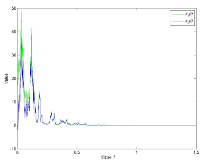
Remark 5.2. It should be pointed out that in Example 5.2 the variable coefficients c_i(t) = 0 for t = \frac{\pi}{2}+2k\pi , k\in \mathbb{N} . This means that the results in [12,23] cannot solve this case.
To compare to some known results, we consider the following SDHNNs which are the special case of [12,16,20,21,22,23].
Example 5.3.
| \begin{eqnarray} \left\{ \begin{array}{ll}dz_i(t) = \bigg[-c_iz_i(t)+\sum\limits_{j = 1}^2a_{ij}f_j(z_j(t))+\sum\limits_{j = 1}^2b_{ij}g_j(z_j(t-\delta_{ij}(t)))\bigg]dt+\sigma_{i}(z_i(t))dw_i(t),\quad t\geq 0,\\ z_i(t) = \phi_i(t),\quad t\in[-1,0],\quad i\in\mathbb{N}_2, \end{array} \right. \end{eqnarray} | (5.3) |
where c_1 = 2 , c_2 = 4 , a_{11} = 0.5 , a_{12} = 1 , b_{11} = 0.25 , b_{12} = 0.5 , a_{21} = \frac{1}{3} , a_{22} = \frac{2}{3} , b_{21} = \frac{1}{3} , b_{22} = \frac{2}{3} , f_1(u) = f_2(u) = arctanu , g_1(u) = g_2(u) = 0.5(|u+1|-|u-1|) , \sigma_{1}(u) = 0.5u , \sigma_{2}(u) = 0.5u , \delta_{11}(t) = \delta_{21}(t) = \delta_{12}(t) = \delta_{22}(t) = 1 , and \phi(t) = (40, 20) for t\in[-1, 0] .
Choose c(t) = 1 , and then \sup\limits_{t\geq0}\int^t_{t-1}\big(1)^*ds = 1 . We can find F_1 = F_2 = G_1 = G_2 = 1 , \rho^{(1)}_{11} = \frac{3}{8} , \rho^{(1)}_{12} = \frac{3}{4} , \rho^{(1)}_{21} = \frac{1}{6} , \rho^{(1)}_{22} = \frac{1}{3} , \rho^{(2)}_{11} = \frac{1}{8} , \rho^{(2)}_{12} = \rho^{(2)}_{21} = 0 , and \rho^{(2)}_{22} = \frac{1}{16} . Then
| \begin{equation*} \rho{ \left( \begin{array}{ccc} \rho_{11}^{(1)}+0.5\rho_{12}^{(1)}+0.5\rho_{11}^{(2)} & 0.5\rho_{12}^{(1)}+0.5\rho_{12}^{(2)} \\ 0.5\rho_{21}^{(1)}+0.5\rho_{21}^{(2)}& \rho_{22}^{(1)}+0.5\rho_{21}^{(1)}+0.5\rho_{22}^{(2)} \end{array} \right )} = \rho{ \left( \begin{array}{ccc} \frac{7}{8} & \frac{3}{8} \\ \frac{1}{12}& \frac{43}{96} \end{array} \right )} < 1. \end{equation*} |
Then (\mathbf{C.1}) – (\mathbf{C.5}) are satisfied (p = 2) . So (5.3) is exponentially stable in mean square (see Figure 3).
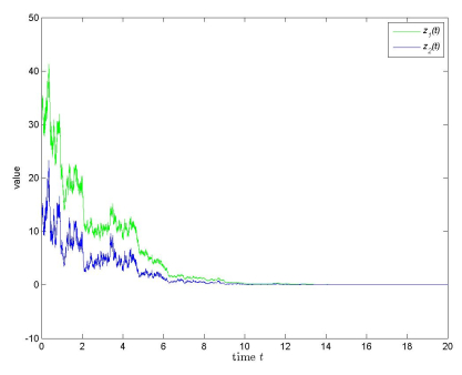
Remark 5.3. It is noteworthy that in Example 5.3,
| \begin{equation*} \rho{ \left( \begin{array}{ccc} \frac{4(a_{11}^2F_1^2+a_{12}^2F_2^2+b_{11}^2G_1^2+b_{12}^2G_2^2)}{c^2_1}+\frac{4\mu_{11}}{c_1} & 0 \\ 0& \frac{4(a_{21}^2F_1^2+a_{22}^2F_2^2+b_{21}^2G_1^2+b_{22}^2G_2^2)}{c^2_2}+\frac{4\mu_{22}}{c_2} \end{array} \right )} = \rho{ \left( \begin{array}{ccc} \frac{33}{16} & 0 \\ 0& \frac{19}{36} \end{array} \right )} = \frac{33}{16} > 1, \end{equation*} |
which makes the result in [20,21,22] invalid. In addition,
| \begin{aligned} \frac{4(a_{11}^2F_1^2+a_{12}^2F_2^2+b_{11}^2G_1^2+b_{12}^2G_2^2)}{c^2_1}+\frac{4(a_{21}^2F_1^2+a_{22}^2F_2^2+b_{21}^2G_1^2+b_{22}^2G_2^2)}{c^2_2} > 1, \end{aligned} |
which makes the result in [16] not applicable in this example. Moreover
| \begin{equation*} -c_1+(a_{11}F_1+a_{12}F_2+b_{11}G_1+b_{11}F_2+\frac{1}{2}\mu_{11}) > 0, \end{equation*} |
which makes the results in [12,23] inapplicable in this example.
In this paper, we have addressed the issue of p th moment generalized exponential stability concerning SHNNs characterized by variable coefficients and infinite delay. Our approach involves the utilization of various inequalities and stochastic analysis techniques. Notably, we have extended and enhanced some existing results. Lastly, we have provided three numerical examples to showcase the practical utility and effectiveness of our results.
Dehao Ruan: Writing and original draft. Yao Lu: Review and editing. Both of the authors have read and approved the final version of the manuscript for publication.
The authors declare they have not used Artificial Intelligence (AI) tools in the creation of this article.
This research was funded by the Talent Special Project of Guangdong Polytechnic Normal University (2021SDKYA053 and 2021SDKYA068), and Guangzhou Basic and Applied Basic Research Foundation (2023A04J0031 and 2023A04J0032).
The authors declare that they have no competing interests.
| [1] |
W. O. Kermack, A. G. McKendrick, A contribution to the mathematical theory of epidemics, Math. Phys. Eng. Sci., 115 (1927), 700–721. https://doi.org/10.1098/rspa.1927.0118 doi: 10.1098/rspa.1927.0118

|
| [2] |
M. Barro, A. Guiro, D. Quedraogo, Optimal control of a SIR epidemic model with general incidence function and a time delays, CUBO A Math. J., 20 (2018), 53–66. https://doi.org/10.4067/S0719-06462018000200053 doi: 10.4067/S0719-06462018000200053
|
| [3] |
P. A. Bliman, M. Duprez, Y. Privat, N. Vauchelet, Optimal immunity control and final size minimization by social distancing for the SIR epidemic model, J. Optim. Theory Appl., 189 (2021), 408–436. https://doi.org/10.1007/s10957-021-01830-1 doi: 10.1007/s10957-021-01830-1
|
| [4] |
L. Bolzoni, E. Bonacini, C. Soresina, M. Groppi, Time-optimal control strategies in SIR epidemic models, Math. Biosci., 292 (2017), 86–96. https://doi.org/10.1016/j.mbs.2017.07.011 doi: 10.1016/j.mbs.2017.07.011
|
| [5] |
E. V. Grigorieva, E. N. Khailov, A. Korobeinikov, Optimal control for a SIR epidemic model with nonlinear incidence rate, Math. Model. Nat. Phenom., 11 (2016), 89–104. https://doi.org/10.1051/mmnp/201611407 doi: 10.1051/mmnp/201611407
|
| [6] |
R. Hynd, D. Ikpe, T. Pendleton, An eradication time problem for the SIR model, J. Differ. Equations, 303 (2021), 214–252. https://doi.org/10.1016/j.jde.2021.09.001 doi: 10.1016/j.jde.2021.09.001
|
| [7] |
R. Hynd, D. Ikpe, T. Pendleton, Two critical times for the SIR model, J. Math. Anal. Appl., 505 (2022), 125507. https://doi.org/10.1016/j.jmaa.2021.125507 doi: 10.1016/j.jmaa.2021.125507
|
| [8] | L. S. Pontryagin, Mathematical Theory of Optimal Processes, Routledge, 2018. |
| [9] | J. Jang, Y. Kim, On a minimum eradication time for the SIR model with time-dependent coefficients, preprint, arXiv: 2311.14657. https://doi.org/10.48550/arXiv.2311.14657 |
| [10] | H. V. Tran, Hamilton-Jacobi equations: Theory and applications, Am. Math. Soc., 213 (2021), 322. |
| [11] |
S. Ko, S. Park, VS-PINN: A fast and efficient training of physics-informed neural networks using variable-scaling methods for solving PDEs with stiff behavior, J. Comput. Phys., 529 (2025), 113860. https://doi.org/10.1016/j.jcp.2025.113860 doi: 10.1016/j.jcp.2025.113860
|
| [12] | A. Jacot, F. Gabriel, C. Hongler, Neural tangent kernel: Convergence and generalization in neural networks, in STOC 2021: Proceedings of the 53rd Annual ACM SIGACT Symposium on Theory of Computing, (2021). https://doi.org/10.1145/3406325.3465355 |
| [13] |
M. Raissi, P. Perdikaris, G. E. Karniadakis, Physics-informed neural networks: A deep learning framework for solving forward and inverse problems involving nonlinear partial differential equations, J. Comput. Phys., 378 (2019), 686–707. https://doi.org/10.1016/j.jcp.2018.10.045 doi: 10.1016/j.jcp.2018.10.045
|
| [14] |
E. Kharazmi, M. Cai, X. Zheng, G. Lin, G. E. Karniadakis, Identifiability and predictability of integer-and fractional-order epidemiological models using physics-informed neural networks, Nat. Comput. Sci., 1 (2021), 744–753. https://doi.org/10.1038/s43588-021-00158-0 doi: 10.1038/s43588-021-00158-0
|
| [15] |
A. Yazdani, L. Lu, M. Raissi, G. E. Karniadakis, Systems biology informed deep learning for inferring parameters and hidden dynamics, PLoS Comput. Biol., 16 (2020), e1007575. https://doi.org/10.1371/journal.pcbi.1007575 doi: 10.1371/journal.pcbi.1007575
|
| [16] |
S. Cai, Z. Mao, Z. Wang, M. Yin, G. E. Karniadakis, Physics-informed neural networks (PINNs) for fluid mechanics: A review, Acta Mech. Sin., 37 (2021), 1727–1738. https://doi.org/10.1007/s10409-021-01148-1 doi: 10.1007/s10409-021-01148-1
|
| [17] |
M. Raissi, A. Yazdani, G. E. Karniadakis, Hidden fluid mechanics: Learning velocity and pressure fields from flow visualizations, Science, 367 (2020), 1026–1030. https://doi.org/10.1126/science.aaw4741 doi: 10.1126/science.aaw4741
|
| [18] |
X. Jin, S. Cai, H. Li, G. E. Karniadakis, NSFnets (Navier-Stokes flow nets): Physics-informed neural networks for the incompressible Navier-Stokes equations, J. Comput. Phys., 426 (2021), 109951. https://doi.org/10.1016/j.jcp.2020.109951 doi: 10.1016/j.jcp.2020.109951
|
| [19] |
X. Wang, J. Li, J. Li, A deep learning based numerical PDE method for option pricing, Comput. Econ., 62 (2023), 149–164. https://doi.org/10.1007/s10614-022-10279-x doi: 10.1007/s10614-022-10279-x
|
| [20] |
Y. Bai, T. Chaolu, S. Bilige, The application of improved physics-informed neural network (IPINN) method in finance, Nonlinear Dyn., 107 (2022), 3655–3667. https://doi.org/10.1007/s11071-021-07146-z doi: 10.1007/s11071-021-07146-z
|
| [21] |
G. Kissas, Y. Yang, E. Hwuang, W. R. Witschey, J. A. Detre, P. Perdikaris, Machine learning in cardiovascular flows modeling: Predicting arterial blood pressure from non-invasive 4d flow MRI data using physics-informed neural networks, Comput. Methods Appl. Mech. Eng., 358 (2020), 112623. https://doi.org/10.1016/j.cma.2019.112623 doi: 10.1016/j.cma.2019.112623
|
| [22] |
F. Sahli C., Y. Yang, P. Perdikaris, D. E. Hurtado, E. Kuhl, Physics-informed neural networks for cardiac activation mapping, Front. Phys., 8 (2020), 42. https://doi.org/10.3389/fphy.2020.00042 doi: 10.3389/fphy.2020.00042
|
| [23] |
S. Wang, Y. Teng, P. Perdikaris, Understanding and mitigating gradient flow pathologies in physics-informed neural networks, SIAM J. Sci. Comput., 43 (2021), A3055–A3081. https://doi.org/10.1137/20M1318043 doi: 10.1137/20M1318043
|
| [24] |
Y. Liu, L. Cai, Y. Chen, B. Wang, Physics-informed neural networks based on adaptive weighted loss functions for Hamilton–Jacobi equations, Math. Biosci. Eng., 19 (2022), 12866–12896. https://doi.org/10.3934/mbe.2022601 doi: 10.3934/mbe.2022601
|
| [25] |
S. Wang, X. Yu, P. Perdikaris, When and why PINNs fail to train: A neural tangent kernel perspective, J. Comput. Phys., 449 (2022), 110768. https://doi.org/10.1016/j.jcp.2021.110768 doi: 10.1016/j.jcp.2021.110768
|
| [26] |
W. Ji, W. Qiu, Z. Shi, S. Pan, S. Deng, Stiff-pinn: Physics-informed neural network for stiff chemical kinetics, J. Phys. Chem. A, 125 (2021), 8098–8106. https://doi.org/10.1021/acs.jpca.1c05102 doi: 10.1021/acs.jpca.1c05102
|
| [27] |
L. D. McClenny, U. M. Braga-Neto, Self-adaptive physics-informed neural networks, J. Comput. Phys., 474 (2023), 111722. https://doi.org/10.1016/j.jcp.2022.111722 doi: 10.1016/j.jcp.2022.111722
|
| [28] |
S. Mowlavi, S. Nabi, Optimal control of PDEs using physics-informed neural networks, J. Comput. Phys., 473 (2023), 111731. https://doi.org/10.1016/j.jcp.2022.111731 doi: 10.1016/j.jcp.2022.111731
|
| [29] | Y. Meng, R. Zhou, A. Mukherjee, M. Fitzsimmons, C. Song, J. Liu, Physics-informed neural network policy iteration: Algorithms, convergence, and verification, preprint, arXiv: 2402.10119. https://doi.org/10.48550/arXiv.2402.10119 |
| [30] | J. Y. Lee, Y. Kim, Hamilton-Jacobi based policy-iteration via deep operator learning, preprint, arXiv: 2406.10920. https://doi.org/10.48550/arXiv.2406.10920 |
| [31] |
W. Tang, H. Tran, Y. Zhang, Policy iteration for the deterministic control problems—A viscosity approach, SIAM J. Control Optim., 63 (2025), 375–401. https://doi.org/10.1137/24M1631602 doi: 10.1137/24M1631602
|
| [32] |
S. Yin, J. Wu, P. Song, Optimal control by deep learning techniques and its applications on epidemic models, J. Math. Biol., 86 (2023), 36. https://doi.org/10.1007/s00285-023-01873-0 doi: 10.1007/s00285-023-01873-0
|
| [33] |
Y. Ye, A. Pandey, C. Bawden, D. Sumsuzzman, R. Rajput, A. Shoukat, et al., Integrating artificial intelligence with mechanistic epidemiological modeling: A scoping review of opportunities and challenges, Nat. Commun., 16 (2025), 581. https://doi.org/10.1038/s41467-024-55461-x doi: 10.1038/s41467-024-55461-x
|
| [34] |
Z. Yang, Z. Zeng, K. Wang, S. Wong, W. Liang, M. Zanin, et al., Modified SEIR and AI prediction of the epidemics trend of COVID-19 in china under public health interventions, J. Thorac. Dis., 12 (2020), 165. https://doi.org/10.21037/jtd.2020.02.64 doi: 10.21037/jtd.2020.02.64
|
| [35] | L. Evans, Partial differential equations: 2nd edition, in Graduate Studies in Mathematics, Am. Math. Soc., 19 (2010), 749. |
| [36] | R. V. Hogg, J. W. McKean, A. T. Craig, Introduction to Mathematical Statistics, 8th edition, 2013. |
| [37] | D. Kingma, Adam: A method for stochastic optimization, preprint, arXiv: 1412.6980. |
Figures(11) / Tables(3)

Minseok Kim, Yeongjong Kim, Yeoneung Kim. Physics-informed neural networks for optimal vaccination plan in SIR epidemic models[J]. Mathematical Biosciences and Engineering, 2025, 22(7): 1598-1633. doi: 10.3934/mbe.2025059

 DownLoad:
