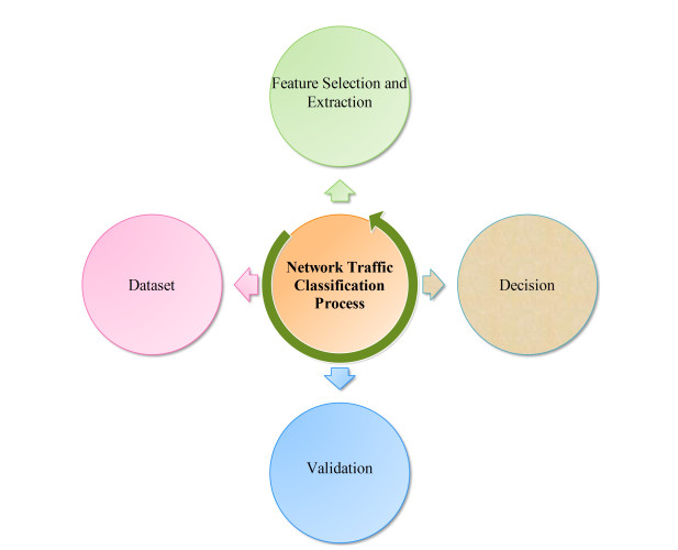
Traditional network analysis frequently relied on manual examination or predefined patterns for the detection of system intrusions. As soon as there was increase in the evolution of the internet and the sophistication of cyber threats, the ability for the identification of attacks promptly became more challenging. Network traffic classification is a multi-faceted process that involves preparation of datasets by handling missing and redundant values. Machine learning (ML) models have been employed to classify network traffic effectively. In this article, we introduce a hybrid Deep learning (DL) model which is designed for enhancing the accuracy of network traffic classification (NTC) within the domain of cyber-physical systems (CPS). Our novel model capitalizes on the synergies among CPS, network traffic classification (NTC), and DL techniques. The model is implemented and evaluated in Python, focusing on its performance in CPS-driven network security. We assessed the model's effectiveness using key metrics such as accuracy, precision, recall, and F1-score, highlighting its robustness in CPS-driven security. By integrating sophisticated hybrid DL algorithms, this research contributes to the resilience of network traffic classification in the dynamic CPS environment.
Citation: Shivani Gaba, Ishan Budhiraja, Vimal Kumar, Aaisha Makkar. Advancements in enhancing cyber-physical system security: Practical deep learning solutions for network traffic classification and integration with security technologies[J]. Mathematical Biosciences and Engineering, 2024, 21(1): 1527-1553. doi: 10.3934/mbe.2024066
Traditional network analysis frequently relied on manual examination or predefined patterns for the detection of system intrusions. As soon as there was increase in the evolution of the internet and the sophistication of cyber threats, the ability for the identification of attacks promptly became more challenging. Network traffic classification is a multi-faceted process that involves preparation of datasets by handling missing and redundant values. Machine learning (ML) models have been employed to classify network traffic effectively. In this article, we introduce a hybrid Deep learning (DL) model which is designed for enhancing the accuracy of network traffic classification (NTC) within the domain of cyber-physical systems (CPS). Our novel model capitalizes on the synergies among CPS, network traffic classification (NTC), and DL techniques. The model is implemented and evaluated in Python, focusing on its performance in CPS-driven network security. We assessed the model's effectiveness using key metrics such as accuracy, precision, recall, and F1-score, highlighting its robustness in CPS-driven security. By integrating sophisticated hybrid DL algorithms, this research contributes to the resilience of network traffic classification in the dynamic CPS environment.

| [1] | J. Guo, M. Cui, C. Hou, G. Gou, Z. Li, G. Xiong, et al., Global-aware prototypical network for few-shot encrypted traffic classification, in 2022 IFIP Networking Conference (IFIP Networking), (2022), 1–9. https://doi.org/10.23919/IFIPNetworking55013.2022.9829771 |
| [2] |
S. Stryczek, M. Natkaniec, Internet threat detection in smart grids based on network traffic analysis using lstm, if, and svm, Energies, 16 (2023), 329. https://doi.org/10.3390/en16010329 doi: 10.3390/en16010329

|
| [3] | H. Liu, B. Lang, Network traffic classification method supporting unknown protocol detection, in 2021 IEEE 46th Conference on Local Computer Networks (LCN), (2021), 311–314. https://doi.org/10.1109/LCN52139.2021.9525009 |
| [4] |
A. Barnawi, S. Gaba, A. Alphy, A. Jabbari, I. Budhiraja, V. Kumar, et al., A systematic analysis of deep learning methods and potential attacks in internet-of-things surfaces, Neural Comput. Appl., 2023 (2023), 1–16. https://doi.org/10.1007/s00521-023-08634-6 doi: 10.1007/s00521-023-08634-6
|
| [5] |
A. Yadav, S. Gaba, H. Khan, I. Budhiraja, A. Singh, K. K. Singh, Etma: Efficient transformer-based multilevel attention framework for multimodal fake news detection, IEEE Trans. Comput. Soc. Syst., 2023 (2023), forthcoming. https://doi.org/10.1109/TCSS.2023.3255242 doi: 10.1109/TCSS.2023.3255242
|
| [6] | R. Moreira, L. F. Rodrigues, P. F. Rosa, R. L. Aguiar, F. de Oliveira Silva, Packet vision: a convolutional neural network approach for network traffic classification, in 2020 33rd SIBGRAPI Conference on Graphics, Patterns and Images (SIBGRAPI), (2020), 256–263. https://doi.org/10.1109/SIBGRAPI51738.2020.00042 |
| [7] | K. Lin, X. Xu, Y. Jiang, A new semi-supervised approach for network encrypted traffic clustering and classification, in 2022 IEEE 25th International Conference on Computer Supported Cooperative Work in Design (CSCWD), (2022), 41–46. https://doi.org/10.1109/CSCWD54268.2022.9776310 |
| [8] |
J. Zhao, X. Liu, Q. Yan, B. Li, M. Shao, H. Peng, Multi-attributed heterogeneous graph convolutional network for bot detection, Inf. Sci., 537 (2020), 380–393. https://doi.org/10.1016/j.ins.2020.03.113 doi: 10.1016/j.ins.2020.03.113
|
| [9] | P. Singh, G. Bathla, D. Panwar, A. Aggarwal, S. Gaba, Performance evaluation of genetic algorithm and flower pollination algorithm for scheduling tasks in cloud computing, in International Conference on Signal Processing and Integrated Networks, (2022), 139–154. https://doi.org/10.1007/978-981-99-1312-1_12 |
| [10] |
S. Gaba, I. Budhiraja, V. Kumar, S. Garg, G. Kaddoum, M. M. Hassan, A federated calibration scheme for convolutional neural networks: Models, applications and challenges, Comput. Commun., 192 (2022), 144–162. https://doi.org/10.1016/j.comcom.2022.05.035 doi: 10.1016/j.comcom.2022.05.035
|
| [11] | A. Aggarwal, S. Gaba, J. Kumar, S. Nagpal, Blockchain and autonomous vehicles: Architecture, security and challenges, in 2022 Fifth International Conference on Computational Intelligence and Communication Technologies (CCICT), IEEE, (2022), 332–338. https://doi.org/10.1109/CCiCT56684.2022.00067 |
| [12] |
Y. Wang, X. Yun, Y. Zhang, C. Zhao, X. Liu, A multi-scale feature attention approach to network traffic classification and its model explanation, IEEE Trans. Network Serv. Manage., 19 (2022), 875–889. https://doi.org/10.1109/TNSM.2022.3149933 doi: 10.1109/TNSM.2022.3149933
|
| [13] |
J. Zhao, M. Shao, H. Wang, X. Yu, B. Li, X. Liu, Cyber threat prediction using dynamic heterogeneous graph learning, Knowl. Based Syst., 240 (2022), 108086. https://doi.org/10.1016/j.knosys.2021.108086 doi: 10.1016/j.knosys.2021.108086
|
| [14] | Q. Ma, W. Huang, Y. Jin, J. Mao, Encrypted traffic classification based on traffic reconstruction, in 2021 4th International Conference on Artificial Intelligence and Big Data (ICAIBD), IEEE, (2021), 572–576. https://doi.org/10.1109/ICAIBD51990.2021.9459072 |
| [15] | Y. Zeng, Z. Qi, W. Chen, Y. Huang, Test: an end-to-end network traffic classification system with spatio-temporal features extraction, in 2019 IEEE International Conference on Smart Cloud (SmartCloud), IEEE, (2019), 131–136. https://doi.org/10.1109/SmartCloud.2019.00032 |
| [16] | A. Aggarwal, S. Gaba, S. Nagpal, A. Arya, A deep analysis on the role of deep learning models using generative adversarial networks, in Blockchain and Deep Learning: Future Trends and Enabling Technologies, Springer, (2022), 179–197. https://doi.org/10.1007/978-3-030-95419-2_9 |
| [17] | S. Nagpal, A. Aggarwal, S. Gaba, Privacy and security issues in vehicular ad hoc networks with preventive mechanisms, in Proceedings of International Conference on Intelligent Cyber-Physical Systems: ICPS 2021, Springer, (2022), 317–329. https://doi.org/10.1007/978-981-16-7136-4_24 |
| [18] |
G. Aceto, D. Ciuonzo, A. Montieri, A. Pescapé, Mobile encrypted traffic classification using deep learning: Experimental evaluation, lessons learned, and challenges, IEEE Trans. Network Serv. Manage., 16 (2019), 445–458. https://doi.org/10.1109/TNSM.2019.2899085 doi: 10.1109/TNSM.2019.2899085
|
| [19] |
M. Lotfollahi, M. J. Siavoshani, R. S. Hossein Zade, M. Saberian, Deep packet: A novel approach for encrypted traffic classification using deep learning, Soft Comput., 24 (2020), 1999–2012. https://doi.org/10.1007/s00500-019-04030-2 doi: 10.1007/s00500-019-04030-2
|
| [20] |
G. Aceto, D. Ciuonzo, A. Montieri, A. Pescapé, MIMETIC: Mobile encrypted traffic classification using multimodal deep learning, Comput. Networks, 165 (2019), 106944. https://doi.org/10.1016/j.comnet.2019.106944 doi: 10.1016/j.comnet.2019.106944
|
| [21] |
M. Lopez-Martin, B. Carro, A. Sanchez-Esguevillas, J. Lloret, Network traffic classifier with convolutional and recurrent neural networks for Internet of Things, IEEE Access, 5 (2017), 18042–18050. https://doi.org/10.1109/ACCESS.2017.2747560 doi: 10.1109/ACCESS.2017.2747560
|
| [22] | J. Li, V. S. Sheng, Z. Shu, Y. Cheng, Y. Jin, Y. F. Yan, Learning from the crowd with neural network, in 2015 IEEE 14th International Conference on Machine Learning and Applications (ICMLA), (2015), 693–698. https://doi.org/10.1109/ICMLA.2015.14 |
| [23] |
X. Y. Zhang, G. S. Xie, C. L. Liu, Y. Bengio, End-to-end online writer identification with recurrent neural network, IEEE Trans. Human Mach. Syst., 47 (2016), 285–292. https://doi.org/10.1109/THMS.2016.2634921 doi: 10.1109/THMS.2016.2634921
|
| [24] |
X. Shi, H. Qi, Y. Shen, G. Wu, B. Yin, A spatial–temporal attention approach for traffic prediction, IEEE Trans. Intell. Transp. Syst., 22 (2020), 4909–4918. https://doi.org/10.1109/TITS.2020.2983651 doi: 10.1109/TITS.2020.2983651
|
| [25] |
Y. Saadna, A. Behloul, An overview of traffic sign detection and classification methods, Int. J. Multimedia Inf. Retr., 6 (2017), 193–210. https://doi.org/10.1007/s13735-017-0129-8 doi: 10.1007/s13735-017-0129-8
|
| [26] |
D. Kaur, A. Anwar, I. Kamwa, S. Islam, S. M. Muyeen, N. Hosseinzadeh, A Bayesian deep learning approach with convolutional feature engineering to discriminate cyber-physical intrusions in smart grid systems, IEEE Access, 11 (2023), 18910–18920. https://doi.org/10.1109/ACCESS.2023.3247947 doi: 10.1109/ACCESS.2023.3247947
|
| [27] |
A. Aldweesh, A. Derhab, A. Z. Emam, Deep learning approaches for anomaly-based intrusion detection systems: A survey, taxonomy, and open issues, Knowl. Based Syst., 189 (2020), 105124. https://doi.org/10.1016/j.knosys.2019.105124 doi: 10.1016/j.knosys.2019.105124
|
| [28] |
J. Bhardwaj, J. P. Krishnan, D. F. L. Marin, B. Beferull-Lozano, L. R. Cenkeramaddi, C. Harman, Cyber-physical systems for smart water networks: A review, IEEE Sens. J., 21 (2021), 26447–26469. https://doi.org/10.1109/JSEN.2021.3121506 doi: 10.1109/JSEN.2021.3121506
|
| [29] |
M. S. Akhtar, T. Feng, Detection of malware by deep learning as CNN-LSTM machine learning techniques in real time, Symmetry, 14 (2022), 2308. https://doi.org/10.3390/sym14112308 doi: 10.3390/sym14112308
|
| [30] | D. D. Godsey, Y. H. Hu, M. A. Hoppa, A Multi-layered Approach to Fake News Identification, Measurement and Mitigation, in Advances in Information and Communication: Proceedings of the 2021 Future of Information and Communication Conference (FICC), (2021), 624–642. https://doi.org/10.1007/978-3-030-73100-7_45 |
| [31] |
Y. Jang, N. Kim, B. D. Lee, Traffic classification using distributions of latent space in software-defined networks: An experimental evaluation, Eng. Appl. Artif. Intell., 119 (2023), 105736. https://doi.org/10.1016/j.engappai.2022.105736 doi: 10.1016/j.engappai.2022.105736
|
| [32] | A. V. Jain, Network traffic identification with convolutional neural networks, in 2018 IEEE 16th Intl Conf on Dependable, Autonomic and Secure Computing, 16th Intl Conf on Pervasive Intelligence and Computing, 4th Intl Conf on Big Data Intelligence and Computing and Cyber Science and Technology Congress (DASC/PiCom/DataCom/CyberSciTech), IEEE, (2018), 1001–1007. |
| [33] |
S. Dong, Multi class svm algorithm with active learning for network traffic classification, Expert Syst. Appl., 176 (2021), 114885. https://doi.org/10.1016/j.eswa.2021.114885 doi: 10.1016/j.eswa.2021.114885
|
| [34] | Y. Guo, G. Xiong, Z. Li, J. Shi, M. Cui, G. Gou, Combating imbalance in network traffic classification using gan based oversampling, in 2021 IFIP Networking Conference (IFIP Networking), IEEE, (2021), 1–9. https://doi.org/10.23919/IFIPNetworking52078.2021.9472777 |
| [35] | F. Al-Obaidy, S. Momtahen, M. F. Hossain, F. Mohammadi, Encrypted traffic classification based ml for identifying different social media applications, in 2019 IEEE Canadian Conference of Electrical and Computer Engineering (CCECE), IEEE, (2019), 1–5. https://doi.org/10.1109/CCECE.2019.8861934 |
| [36] |
X. Ren, H. Gu, W. Wei, Tree-rnn: Tree structural recurrent neural network for network traffic classification, Expert Syst. Appl., 167 (2021), 114363. https://doi.org/10.1016/j.eswa.2020.114363 doi: 10.1016/j.eswa.2020.114363
|
| [37] |
W. Liu, C. Zhu, Z. Ding, H. Zhang, Q. Liu, Multiclass imbalanced and concept drift network traffic classification framework based on online active learning, Eng. Appl. Artif. Intell., 117 (2023), 105607. https://doi.org/10.1016/j.engappai.2022.105607 doi: 10.1016/j.engappai.2022.105607
|
| [38] |
Y. Pan, X. Zhang, H. Jiang, C. Li, A network traffic classification method based on graph convolution and lstm, IEEE Access, 9 (2021), 158261–158272. https://doi.org/10.1109/ACCESS.2021.3128181 doi: 10.1109/ACCESS.2021.3128181
|
| [39] |
C. Gijón, M. Toril, M. Solera, S. Luna-Ramírez, L. R. Jimenez, Encrypted traffic classification based on unsupervised learning in cellular radio access networks, IEEE Access, 8 (2020), 167252–167263. https://doi.org/10.1109/ACCESS.2020.3022980 doi: 10.1109/ACCESS.2020.3022980
|
| [40] |
X. Jing, J. Zhao, Z. Yan, W. Pedrycz, X. Li, Granular classifier: Building traffic granules for encrypted traffic classification based on granular computing, Dig. Commun. Networks, 2022 (2022), forthcoming. https://doi.org/10.1016/j.dcan.2022.12.017 doi: 10.1016/j.dcan.2022.12.017
|
| [41] |
S. Ahn, J. Kim, S. Y. Park, S. Cho, Explaining deep learning-based traffic classification using a genetic algorithm, IEEE Access, 9 (2020), 4738–4751. https://doi.org/10.1109/ACCESS.2020.3048348 doi: 10.1109/ACCESS.2020.3048348
|
| [42] | J. Zhang, J. Zhou, N. Zhou, Network traffic classification method based on subspace triple attention mechanism, in 2022 3rd International Conference on Information Science, Parallel and Distributed Systems (ISPDS), IEEE, (2022), 312–316. https://doi.org/10.1109/ISPDS56360.2022.9874195 |
| [43] |
A. S. Iliyasu, H. Deng, Semi-supervised encrypted traffic classification with deep convolutional generative adversarial networks, IEEE Access, 8 (2019), 118–126. https://doi.org/10.1109/ACCESS.2019.2962106 doi: 10.1109/ACCESS.2019.2962106
|
| [44] |
L. K. Ramasamy, F. Khan, M. Shah, B. V. V. S. Prasad, C. Iwendi, C. Biamba, Secure smart wearable computing through artificial intelligence-enabled internet of things and cyber-physical systems for health monitoring, Sensors, 22 (2022), 1076. https://doi.org/10.3390/s22031076 doi: 10.3390/s22031076
|
Figures(10) / Tables(3)

Shivani Gaba, Ishan Budhiraja, Vimal Kumar, Aaisha Makkar. Advancements in enhancing cyber-physical system security: Practical deep learning solutions for network traffic classification and integration with security technologies[J]. Mathematical Biosciences and Engineering, 2024, 21(1): 1527-1553. doi: 10.3934/mbe.2024066


 DownLoad: