An Alzheimer's Disease classification network based on MRI utilizing diffusion maps for multi-scale feature fusion in graph convolution

Zhi Yang; Kang Li; Haitao Gan; Zhongwei Huang; Ming Shi; Ran Zhou; Zhi Yang; Kang Li; Haitao Gan; Zhongwei Huang; Ming Shi; Ran Zhou

doi:10.3934/mbe.2024067

Mathematical Biosciences and Engineering

2024, Volume 21, Issue 1: 1554-1572. doi: 10.3934/mbe.2024067

Previous Article Next Article

Research article

An Alzheimer's Disease classification network based on MRI utilizing diffusion maps for multi-scale feature fusion in graph convolution

School of Computer Science, Hubei University of Technology, Wuhan 430068, China

Received: 07 October 2023 Revised: 19 December 2023 Accepted: 21 December 2023 Published: 29 December 2023

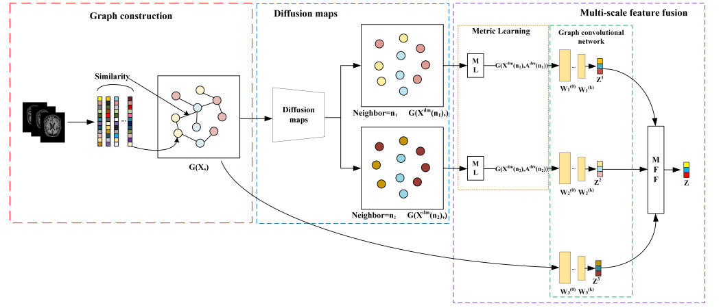
Graph convolutional networks (GCN) have been widely utilized in Alzheimer's disease (AD) classification research due to its ability to automatically learn robust and powerful feature representations. Inter-patient relationships are effectively captured by constructing patients magnetic resonance imaging (MRI) data as graph data, where nodes represent individuals and edges denote the relationships between them. However, the performance of GCNs might be constrained by the construction of the graph adjacency matrix, thereby leading to learned features potentially overlooking intrinsic correlations among patients, which ultimately causes inaccurate disease classifications. To address this issue, we propose an Alzheimer's disease Classification network based on MRI utilizing diffusion maps for multi-scale feature fusion in graph convolution. This method aims to tackle the problem of features neglecting intrinsic relationships among patients while integrating features from diffusion mapping with different neighbor counts to better represent patients and achieve an accurate AD classification. Initially, the diffusion maps method conducts diffusion information in the feature space, thus breaking free from the constraints of diffusion based on the adjacency matrix. Subsequently, the diffusion features with different neighbor counts are merged, and a self-attention mechanism is employed to adaptively adjust the weights of diffusion features at different scales, thereby comprehensively and accurately capturing patient characteristics. Finally, metric learning techniques enhance the similarity of node features within the same category in the graph structure and bring node features of different categories more distant from each other. This study aims to enhance the classification accuracy of AD, by providing an effective tool for early diagnosis and intervention. It offers valuable information for clinical decisions and personalized treatment. Experimentation on the publicly accessible Alzheimer's disease neuroimaging initiative (ADNI) dataset validated our method's competitive performance across various AD-related classification tasks. Compared to existing methodologies, our approach captures patient characteristics more effectively and demonstrates superior generalization capabilities.
- Alzheimer's disease,
- graph convolutional network,
- deep learning,
- diffusion maps,
- metric learning
Citation: Zhi Yang, Kang Li, Haitao Gan, Zhongwei Huang, Ming Shi, Ran Zhou. An Alzheimer's Disease classification network based on MRI utilizing diffusion maps for multi-scale feature fusion in graph convolution[J]. Mathematical Biosciences and Engineering, 2024, 21(1): 1554-1572. doi: 10.3934/mbe.2024067

Related Papers:

Abstract

Graph convolutional networks (GCN) have been widely utilized in Alzheimer's disease (AD) classification research due to its ability to automatically learn robust and powerful feature representations. Inter-patient relationships are effectively captured by constructing patients magnetic resonance imaging (MRI) data as graph data, where nodes represent individuals and edges denote the relationships between them. However, the performance of GCNs might be constrained by the construction of the graph adjacency matrix, thereby leading to learned features potentially overlooking intrinsic correlations among patients, which ultimately causes inaccurate disease classifications. To address this issue, we propose an Alzheimer's disease Classification network based on MRI utilizing diffusion maps for multi-scale feature fusion in graph convolution. This method aims to tackle the problem of features neglecting intrinsic relationships among patients while integrating features from diffusion mapping with different neighbor counts to better represent patients and achieve an accurate AD classification. Initially, the diffusion maps method conducts diffusion information in the feature space, thus breaking free from the constraints of diffusion based on the adjacency matrix. Subsequently, the diffusion features with different neighbor counts are merged, and a self-attention mechanism is employed to adaptively adjust the weights of diffusion features at different scales, thereby comprehensively and accurately capturing patient characteristics. Finally, metric learning techniques enhance the similarity of node features within the same category in the graph structure and bring node features of different categories more distant from each other. This study aims to enhance the classification accuracy of AD, by providing an effective tool for early diagnosis and intervention. It offers valuable information for clinical decisions and personalized treatment. Experimentation on the publicly accessible Alzheimer's disease neuroimaging initiative (ADNI) dataset validated our method's competitive performance across various AD-related classification tasks. Compared to existing methodologies, our approach captures patient characteristics more effectively and demonstrates superior generalization capabilities.

References

[1]	G. McKhann, D. Drachman, M. Folstein, R. Katzman, D. Price, E. M. Stadlan, Clinical diagnosis of Alzheimer's disease: Report of the NINCDS-ADRDA Work Group* under the auspices of Department of Health and Human Services Task Force on Alzheimer's disease, Neurology, 34 (1984), 939–939. https://doi.org/10.1212/WNL.34.7.939 doi: 10.1212/WNL.34.7.939
[2]	L. F. Jia, M. N. Quan, Y. Fu, T. Zhao, Y. Li, C. B. Wei, et al., Dementia in China: epidemiology, clinical management, and research advances, Lancet Neurol., 19 (2020), 81–92. https://doi.org/10.1016/S1474-4422(19)30290-X doi: 10.1016/S1474-4422(19)30290-X
[3]	Risk reduction of cognitive decline and dementia: WHO guidelines, World Health Organization, 2019. Available from: https://www.who.int/publications-detail-redirect/9789241550543.
[4]	M. Calabrò, C. Rinaldi, G. Santoro, C. Crisafulli, The biological pathways of Alzheimer disease: A review, AIMS Neurosci., 8 (2021), 86–86. https://doi.org/10.3934/Neuroscience.2021005 doi: 10.3934/Neuroscience.2021005
[5]	W. Jagust, Vulnerable neural systems and the borderland of brain aging and neurodegeneration, Neuron, 77 (2013), 219–234. http://dx.doi.org/10.1016/j.neuron.2013.01.002 doi: 10.1016/j.neuron.2013.01.002
[6]	N. Habib, C. McCabe, S. Medina, M. Varshavsky, D. Kitsberg, R. Dvir-Szternfeld, et al., Disease-associated astrocytes in Alzheimer's disease and aging, Nat. Neurosci., 23 (2020), 701–706. https://doi.org/10.1038/s41593-020-0624-8 doi: 10.1038/s41593-020-0624-8
[7]	Alzheimer's Association, 2019 Alzheimer's disease facts and figures, Alzheimer Dementia, 15 (2019), 321–387. https://doi.org/10.1016/j.jalz.2019.01.010 doi: 10.1016/j.jalz.2019.01.010
[8]	J. H. Wen, E. Thibeau-Sutre, M. Diaz-Melo, J. Samper-González, A. Routier, S. Bottani, et al., Convolutional neural networks for classification of Alzheimer's disease: Overview and reproducible evaluation, Med. Image Anal., 63 (2020), 101694. https://doi.org/10.1016/j.media.2020.101694 doi: 10.1016/j.media.2020.101694
[9]	M. H. Liu, F. Li, H. Yan, K. D. Wang, Y. X. Ma, L. Shen, et al., A multi-model deep convolutional neural network for automatic hippocampus segmentation and classification in Alzheimer's disease, Neuroimage, 208 (2020), 116459. https://doi.org/10.1016/j.neuroimage.2019.116459 doi: 10.1016/j.neuroimage.2019.116459
[10]	T. Abuhmed, S. El-Sappagh, J. M. Alonso, Robust hybrid deep learning models for Alzheimer's progression detection, Knowl. Based Syst., 213 (2021), 106688. https://doi.org/10.1016/j.knosys.2020.106688 doi: 10.1016/j.knosys.2020.106688
[11]	A. M. Alvi, S. Siuly, H. Wang, K. Wang, F. Whittaker, A deep learning based framework for diagnosis of mild cognitive impairment, Knowl. Based Syst., 248 (2022), 108815. https://doi.org/10.1016/j.knosys.2022.108815 doi: 10.1016/j.knosys.2022.108815
[12]	X. M. Chen, T. Wang, H. R. Lai, X. L. Zhang, Q. J. Feng, M. Y. Huang, Structure-constrained combination-based nonlinear association analysis between incomplete multimodal imaging and genetic data for biomarker detection of neurodegenerative diseases, Med. Image Anal., 78 (2022), 102419. https://doi.org/10.1016/j.media.2022.102419 doi: 10.1016/j.media.2022.102419
[13]	G. B. Frisoni, N. C. Fox, C. R. Jack Jr, P. Scheltens, P. M. Thompson, The clinical use of structural MRI in Alzheimer disease, Nat. Rev. Neurol., 6 (2010), 67–77. https://doi.org/10.1038/nrneurol.2009.215 doi: 10.1038/nrneurol.2009.215
[14]	P. Cao, X. L. Liu, J. Z. Yang, D. Z. Zhao, M. Huang, J. Zhang, et al., Nonlinearity-aware based dimensionality reduction and over-sampling for AD/MCI classification from MRI measures, Comput. Biol. Med., 91 (2017), 21–37. https://doi.org/10.1016/j.compbiomed.2017.10.002 doi: 10.1016/j.compbiomed.2017.10.002
[15]	K. Bäckström, M. Nazari, I.Y. Gu, A.S. Jakola, An efficient 3D deep convolutional network for Alzheimer's disease diagnosis using MR images, in 2018 IEEE 15th International Symposium on Biomedical Imaging (ISBI 2018), (2018), 149–153. https://doi.org/10.1109/ISBI.2018.8363543
[16]	C. F. Lian, M. X. Liu, L. Wang, D. G. Shen, End-to-end dementia status prediction from brain mri using multi-task weakly-supervised attention network, in Medical Image Computing and Computer Assisted Intervention–MICCAI 2019: 22nd International Conference, Shenzhen, China, October 13–17, 2019, Proceedings, Part IV 22, (2019), 158–167. https://doi.org/10.1007/978-3-030-32251-9_18
[17]	K. Mortensen, T. L. Hughes, Comparing Amazon's Mechanical Turk platform to conventional data collection methods in the health and medical research literature, J. Gene. Intern. Med., 33 (2018), 533–538. https://doi.org/10.1007/s11606-017-4246-0 doi: 10.1007/s11606-017-4246-0
[18]	S. Parisot, S. I. Ktena, E. Ferrante, M. Lee, R. Guerrero, B. Glocker, et al., Disease prediction using graph convolutional networks: application to autism spectrum disorder and Alzheimer's disease, Med. Image Anal., 48 (2018), 117–130. https://doi.org/10.1016/j.media.2018.06.001 doi: 10.1016/j.media.2018.06.001
[19]	L. Peng, R. Y. Hu, F. Kong, J. Z. Gan, Y. J. Mo, X. S. Shi, et al., Reverse graph learning for graph neural network, IEEE Trans. Neural Networks Learn. Syst., (2022). https://doi.org/10.1109/TNNLS.2022.3161030
[20]	Q. Ni, J. C. Ji, B. Halkon, K. Feng, A. K. Nandi, Physics-Informed Residual Network (PIResNet) for rolling element bearing fault diagnostics, Mechan. Syst. Signal Process., 200 (2023), 110544. https://doi.org/10.1016/j.ymssp.2023.110544 doi: 10.1016/j.ymssp.2023.110544
[21]	Y. D. Xu, K. Feng, X. A. Yan, R. Q. Yan, Q. Ni, B. B. Sun, et al., CFCNN: A novel convolutional fusion framework for collaborative fault identification of rotating machinery, Inf. Fusion, 95 (2023), 1–16. https://doi.org/10.1016/j.inffus.2023.02.012 doi: 10.1016/j.inffus.2023.02.012
[22]	Z. Yang, K. Li, H. T. Gan, Z. W. Huang, M. Shi, HD-GCN: A hybrid diffusion graph convolutional network, preprint, arXiv: 2303.17966.
[23]	B. Perozzi, R. Al-Rfou, S. Skiena, Deepwalk: Online learning of social representations, in Proceedings of the 20nd ACM SIGKDD International Conference on Knowledge Discovery and Data Mining, (2014), 701–710. https://doi.org/10.1145/2623330.2623732
[24]	A. Grover, J. Leskovec, node2vec: Scalable feature learning for networks, in Proceedings of the 22nd ACM SIGKDD International Conference on Knowledge Discovery and Data Mining, (2016), 855–864. https://doi.org/10.1145/2939672.2939754
[25]	S. Abu-El-Haija, B. Perozzi, R. Al-Rfou, A. A. Alemi, Watch your step: Learning node embeddings via graph attention, in Advances in Neural Information Processing Systems 31 (NeurIPS 2018), 2018.
[26]	S. Abu-El-Haija, A. Kapoor, B. Perozzi, J. Lee, N-gcn: Multi-scale graph convolution for semi-supervised node classification, Uncertainty Artif. Intell., 2020 (2020), 841–851.
[27]	J. L. Zhu, M. W. Jia, Y. Zhang, W. H. Zhou, H. Y. Deng, Y. Liu, Domain adaptation graph convolution network for quality inferring of batch processes, Chemom. Intell. Lab. Syst., 2023 (2023), 105028. https://doi.org/10.1016/j.chemolab.2023.105028 doi: 10.1016/j.chemolab.2023.105028
[28]	M. W. Jia, D. Y. Xu, T. Yang, Y. Liu, Y. Yao, Graph convolutional network soft sensor for process quality prediction, J. Process Control, 123 (2023), 12–25. https://doi.org/10.1016/j.jprocont.2023.01.010 doi: 10.1016/j.jprocont.2023.01.010
[29]	T. N. Kipf, M. Welling, Semi-supervised classification with graph convolutional networks, preprint, arXiv: 1609.02907.
[30]	D. Liben-Nowell, J. Kleinberg, The link prediction problem for social networks, in Proceedings of the Twelfth International Conference on Information and Knowledge Management, 2003 (2003), 556–559. https://doi.org/10.1145/956863.956972
[31]	A. Fout, J. Byrd, B. Shariat, A. Ben-Hur, Protein interface prediction using graph convolutional networks, in Advances in Neural Information Processing Systems 30 (NIPS 2017), (2017), 1–10.
[32]	T. Hamaguchi, H. Oiwa, M. Shimbo, Y. Matsumoto, Knowledge transfer for out-of-knowledge-base entities: A graph neural network approach, preprint, arXiv: 1706.05674.
[33]	E. Xing, M. Jordan, S. J. Russell, A. Ng, Distance Metric Learning with Application to Clustering with Side-Information, in Advances in Neural Information Processing Systems 15 (NIPS 2002), (2002), 521–528.
[34]	K. Q. Weinberger, J. Blitzer, L. Saul, Distance metric learning for large margin nearest neighbor classification, in Advances in Neural Information Processing Systems 18 (NIPS 2005), (2005), 1473–1480.
[35]	R. Y. Li, S. Wang, F. Y. Zhu, J. Z. Huang, Adaptive graph convolutional neural networks, in Proceedings of the AAAI Conference on Artificial Intelligence, 32 (2018). https://doi.org/10.1609/aaai.v32i1.11691
[36]	S. G. Lv, G. Wen, S. Y. Liu, L. S. Wei, M. Li, Robust graph structure learning with the alignment of features and adjacency matrix, preprint, arXiv: 2307.02126.
[37]	S. Parisot, S. I. Ktena, E. Ferrante, M. Lee, R. Guerrero, B. Glocker, et al., Disease prediction using graph convolutional networks: application to autism spectrum disorder and Alzheimer's disease, Med. Image Anal., 48 (2018), 117–130. https://doi.org/10.1016/j.media.2018.06.001 doi: 10.1016/j.media.2018.06.001
[38]	A. Kazi, S. Shekarforoush, K. Kortuem, S. Albarqouni, N. Navab, Self-attention equipped graph convolutions for disease prediction, in 2019 IEEE 16th International Symposium on Biomedical Imaging (ISBI 2019), (2019), 1896–1899. https://doi.org/10.1109/ISBI.2019.8759274
[39]	A. Kazi, S. Shekarforoush, S. Arvind Krishna, H. Burwinkel, G. Vivar, B. Wiestler, et al., Graph convolution based attention model for personalized disease prediction, in Medical Image Computing and Computer Assisted Intervention, (2019), 122–130. https://doi.org/10.1007/978-3-030-32251-9_14
[40]	A. Kazi, S. Shekarforoush, S. Arvind Krishna, H. Burwinkel, G. Vivar, K. Kortüm, et al., InceptionGCN: receptive field aware graph convolutional network for disease prediction, in Information Processing in Medical Imaging: 26th International Conference, IPMI 2019, (2019), 73–85. https://doi.org/10.1007/978-3-030-20351-1_6
[41]	G. Vivar, A. Zwergal, N. Navab, S. A. Ahmadi, Multi-modal disease classification in incomplete datasets using geometric matrix completion, in Graphs in Biomedical Image Analysis and Integrating Medical Imaging and Non-Imaging Modalities, (2018), 24–31. https://doi.org/10.1007/978-3-030-00689-1_3
[42]	A. Vaswani, N. Shazeer, N. Parmar, J. Uszkoreit, L. Jones, A. N. Gomez, et al., Attention is all you need, in Advances in Neural Information Processing Systems 30 (NIPS 2017), 2017.
[43]	V. Mnih, N. Heess, A. Graves, Recurrent models of visual attention, in Advances in Neural Information Processing Systems 27 (NIPS 2014), 2014.
[44]	C. Cortes, V. Vapnik, Support-vector networks, Mach. Learn., 20 (1995), 273–297. https://doi.org/10.1007/BF00994018 doi: 10.1007/BF00994018
[45]	K. M. He, X. Y. Zhang, S. Q. Ren, J. Sun, Deep residual learning for image recognition, in Proceedings of the IEEE Conference on Computer Vision and Pattern Recognition, (2016), 770–778.
[46]	P. Veličković, G. Cucurull, A. Casanova, A. Romero, P. Lio, Y. Bengio, Graph attention networks, preprint, arXiv: 1710.10903.
[47]	H. Y. Gao, S. W. Ji, Graph u-nets, in international Conference on Machine Learning, (2019), 2083–2092.
[48]	J. Lee, I. Lee, J. Kang, Self-attention graph pooling, in International Conference on Machine Learning, (2019), 3734–3743.
[49]	E. Rossi, B. Charpentier, F. Di Giovanni, F. Frasca, S. Günnemann, M. Bronstein, Edge directionality improves learning on heterophilic graphs, preprint, arXiv: 2305.10498

Reader Comments

Your name:*

Email:*
© 2024 the Author(s), licensee AIMS Press. This is an open access article distributed under the terms of the Creative Commons Attribution License (http://creativecommons.org/licenses/by/4.0)