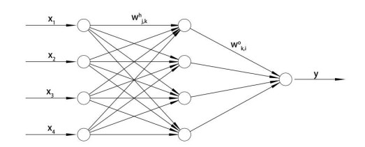
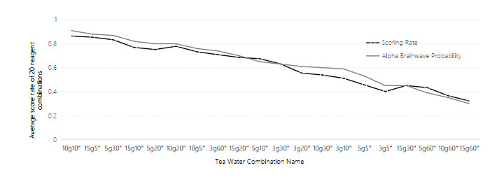
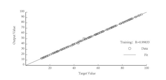
Tea can help to regulate the mood of human. Based on the influence of tea on people's mood and attention, this study explored the tea concentration when the mood and attention of drinkers are in the best state, and established the best concentration model of tea. Using sampling experiment method to collect objective data, which are then combined with questionnaire survey method to collect subjective data, using the results to establish a neural network algorithm model to test the accuracy of the neural network algorithm model. Experiments show that the correlation coefficient of the output value of the BP neural network model constructed in this study is basically consistent with the actual prediction result. After obtaining data such as age, gender, frequency of tea drinking, and tea drinking concentration of tea drinkers, the constructed back propagation (BP) neural network model can accurately predict the mental state score of tea drinkers. The research will provide certain data support and theoretical basis for the follow-up development of the tea industry. Follow-up work needs to be performed in order to further adjust the scope and accuracy of the control model. Then, a more complete and accurate advanced BP neural network model can be established for different types of tea and other parameters.
Citation: Biyun Hong, Yang Zhang. Research on the influence of attention and emotion of tea drinkers based on artificial neural network[J]. Mathematical Biosciences and Engineering, 2021, 18(4): 3423-3434. doi: 10.3934/mbe.2021171
Tea can help to regulate the mood of human. Based on the influence of tea on people's mood and attention, this study explored the tea concentration when the mood and attention of drinkers are in the best state, and established the best concentration model of tea. Using sampling experiment method to collect objective data, which are then combined with questionnaire survey method to collect subjective data, using the results to establish a neural network algorithm model to test the accuracy of the neural network algorithm model. Experiments show that the correlation coefficient of the output value of the BP neural network model constructed in this study is basically consistent with the actual prediction result. After obtaining data such as age, gender, frequency of tea drinking, and tea drinking concentration of tea drinkers, the constructed back propagation (BP) neural network model can accurately predict the mental state score of tea drinkers. The research will provide certain data support and theoretical basis for the follow-up development of the tea industry. Follow-up work needs to be performed in order to further adjust the scope and accuracy of the control model. Then, a more complete and accurate advanced BP neural network model can be established for different types of tea and other parameters.

| [1] | C. Dietz, M. Dekker, B. Piqueras-Fiszman, An intervention study on the effect of matcha tea, in drink and snack bar formats, on mood and cognitive performance, Food Res. Int., 99 (2017), 72-83. |
| [2] | K. L. Spittler, Consumption of green and black tea is associated with a lower risk of stroke, Neurol. Rev., 2009. |
| [3] |
D. Scott, J. A. Rycroft, J. Aspen, C. Chapman, B. Brown, The effect of drinking tea at high altitude on hydration status and mood, Eur. J. Appl. Physiol., 91 (2004), 493-498. doi: 10.1007/s00421-003-1015-z

|
| [4] | N. Khan, H. Mukhtar, Tea polyphenols for health promotion. Life Sci., 81 (2007), 519-533. |
| [5] | T. Mihelj, A. Belscak-Cvitanovic, D. Komes, D. Horzic, V. Tomasic, Bioactive compounds and antioxidant capacity of yellow Yinzhen tea affected by different extraction conditions, J. Food Nutrit. Res., 53 (2014), 278-290. |
| [6] |
D. A. Purwanto, Analysis of ifn-γ concentration in wistar rat blood after oral administration of standardized green tea water extract, Indones. J. Chem., 10 (2010), 390-395. doi: 10.22146/ijc.21448
|
| [7] | M. Rizon, M. Murugappan, R. Nagarajan, S. Yaacob, Asymmetric ratio and FCM based salient channel selection for human emotion detection using EEG, Wseas Trans. Signal Process., 4 (2008), 596-603. |
| [8] |
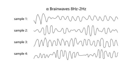
K. Kobayashi, Y. Nagato, N. Aoi, Effect of L-theanine on the release of α-brain waves in human volunteers, Nippon Nogeikagaku Kaishi, 72 (1998), 153-157. doi: 10.1271/nogeikagaku1924.72.153
|
| [9] |
J. Xi, Y. Xue, Y. Xu, Y. Shen, Artificial neural network modeling and optimization of ultrahigh pressure extraction of green tea polyphenols, Food Chem., 141 (2013), 320-326. doi: 10.1016/j.foodchem.2013.02.084
|
| [10] | J. Ning, X. Wan, Z. Zhang, X. Mao, X. Zeng, Discriminating fermentation degree of Puer tea based on NIR spectroscopy and artificial neural network, Trans. Chinese Soc. Agric. Eng., 29 (2013), 255-260. |
| [11] |
N. Das, K. Kalita, P. K. Boruah, U. Sarma, Prediction of moisture loss in withering process of tea manufacturing using artificial neural network, Instrum. Meas., IEEE Trans., 67 (2018), 175-184. doi: 10.1109/TIM.2017.2754818
|
| [12] | Z. C. Guang, L. Y. Chun, Y. Tian, H. C. Quan, S. Xin, A study of identification of taste signals based on fuzzy neural networks. Journal of computer research and development, Comput. Res. Dev., 36 (1999), 18-26. |
| [13] |
H. Lin, Z. Li, H. Lu, S. Sun, F. Chen, K. Wei, et al., Robust classification of tea based on multi-channel LED-induced fluorescence and a convolutional neural network, Sensors (Basel), 19 (2019), 4687. doi: 10.3390/s19214687
|
| [14] | L. I. Yang, L. I. Rui-Rong, L. Y. Wang, Studies on the infusing rules of effective constituents in tea with different water temperature, Beverage Ind., 3 (2015), 1-5. |
| [15] | X. U. Mei-Ling, Measuring the caffeine concentration in green tea beverage by high performance liquid chromatography, Beverage Ind., 3 (2015), 6-9. |
| [16] |
M. Jovović, B. Femić-Radosavović, M. Lipovina-Božović, Comparative analysis of results of online and offline customer satisfaction loyalty surveys in banking services in montenegro, J. Cent. Banking Theory Pract., 6 (2017), 65-76. doi: 10.1515/jcbtp-2017-0013
|
| [17] | R. Marfil, R. Giménez, O. Martínez, P. R. Bouzas, J. Rufián-Henares, M. Mesías, et al., Determination of polyphenols, tocopherols, and antioxidant capacity in virgin argan oil (Argania spinosa, Skeels), European J. Lipid Sci. Technol., 113 (2011), 886-893. |
| [18] | K. Esfahanizadeh, G. Hemati, N. Valaei, Effect of brewing time on the amount of fluoring released from tea, J. Res. Dentalences, 6 (2010), 63-68. |
| [19] |
R. W. Massof, Likert and guttman scaling of visual function rating scale questionnaires, Ophthalmic Epidem., 11 (2004), 381-399. doi: 10.1080/09286580490888771
|
| [20] |
S. E. Harpe, How to analyze likert and other rating scale data, Curr. Pharm. Teach. Learn., 7 (2015), 836-850. doi: 10.1016/j.cptl.2015.08.001
|
| [21] |
E. Cho, S. Kim, Cronbachs coefficient alpha: well known but poorly understood, Organ. Res. Methods, 18 (2015), 207-230. doi: 10.1177/1094428114555994
|
| [22] |
L. J. Cronbach, P. Schonemann, D. Mckie, Alpha coefficients for stratified-parallel tests, Educ. Psychol. Meas., 25 (1965), 291-312. doi: 10.1177/001316446502500201
|
Figures(7) / Tables(6)

Biyun Hong, Yang Zhang. Research on the influence of attention and emotion of tea drinkers based on artificial neural network[J]. Mathematical Biosciences and Engineering, 2021, 18(4): 3423-3434. doi: 10.3934/mbe.2021171


 DownLoad: