The development of the global model is an important part of research involving the quality prediction of agricultural commodities using visible/near-infrared (Vis/NIR) spectroscopy due to its efficiency and effectiveness. The Vis/NIR was used in this study to develop a global model and to evaluate the sugar content and pulp color, which are the main determinants of ripeness and quality of melons. Furthermore, it also provides a comparison between linear and nonlinear regression using partial least squares regression (PLSR) and support vector machine regression (SVMR), respectively. The model accuracy was determined by ratio of performance to deviation (RPD). The results showed that there were good model accuracy values in some parameters, such as SSC (2.14), glucose (1.59), sucrose (2.31), a* (2.97), and b* (2.49), while the fructose (1.35) and L* (1.06) modeling showed poor prediction accuracy. The best model for SSC was developed using PLSR, while that of fructose, glucose, sucrose, L*, a*, and b* were obtained from SVMR. Therefore, Vis/NIR spectroscopy can be used as an alternative method to monitor sugar content and pulp color of a melon, but with some limitations, such as the low accuracy in predicting certain variables, such as the L* and fructose.
Citation: Kusumiyati Kusumiyati, Yuda Hadiwijaya, Wawan Sutari, Agus Arip Munawar. Global model for in-field monitoring of sugar content and color of melon pulp with comparative regression approach[J]. AIMS Agriculture and Food, 2022, 7(2): 312-325. doi: 10.3934/agrfood.2022020
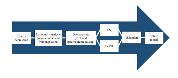
The development of the global model is an important part of research involving the quality prediction of agricultural commodities using visible/near-infrared (Vis/NIR) spectroscopy due to its efficiency and effectiveness. The Vis/NIR was used in this study to develop a global model and to evaluate the sugar content and pulp color, which are the main determinants of ripeness and quality of melons. Furthermore, it also provides a comparison between linear and nonlinear regression using partial least squares regression (PLSR) and support vector machine regression (SVMR), respectively. The model accuracy was determined by ratio of performance to deviation (RPD). The results showed that there were good model accuracy values in some parameters, such as SSC (2.14), glucose (1.59), sucrose (2.31), a* (2.97), and b* (2.49), while the fructose (1.35) and L* (1.06) modeling showed poor prediction accuracy. The best model for SSC was developed using PLSR, while that of fructose, glucose, sucrose, L*, a*, and b* were obtained from SVMR. Therefore, Vis/NIR spectroscopy can be used as an alternative method to monitor sugar content and pulp color of a melon, but with some limitations, such as the low accuracy in predicting certain variables, such as the L* and fructose.

| [1] | Kusumiyati, Hadiwijaya Y, Putri IE, et al. (2021) Multi-product calibration model for soluble solids and water content quantification in Cucurbitaceae family, using visible/near-infrared spectroscopy. Heliyon 7: e07677. https://doi.org/10.1016/j.heliyon.2021.e07677 |
| [2] |
Kusumiyati K, Hadiwijaya Y, Putri IE, et al. (2021) Enhanced visible/near-infrared spectroscopic data for prediction of quality attributes in Cucurbitaceae commodities. Data Brief 39: 107458. https://doi.org/10.1016/j.dib.2021.107458 doi: 10.1016/j.dib.2021.107458

|
| [3] |
Hadiwijaya Y, Kusumiyati K, Munawar AA (2020) Penerapan teknologi visible-near infrared spectroscopy untuk prediksi cepat dan simultan kadar air buah melon (Cucumis melo L.) golden. Agroteknika 3: 67-74. https://doi.org/10.32530/agroteknika.v3i2.83 doi: 10.32530/agroteknika.v3i2.83
|
| [4] | Hadiwijaya Y, Kusumiyati K, Munawar AA (2020) Prediksi total padatan terlarut buah melon golden menggunakan vis-swnirs dan analisis multivariat. J Penelit Saintek 25: 103-114. |
| [5] |
Mancini M, Mazzoni L, Gagliardi F, et al. (2020) Application of the non-destructive NIR technique for the evaluation of strawberry fruits quality parameters. Foods 9: 441. https://doi.org/10.3390/foods9040441 doi: 10.3390/foods9040441
|
| [6] |
Gao Q, Wang ML, Guo YY, et al. (2019) Comparative analysis of non-destructive prediction model of soluble solids content for malus micromalus makino based on near-infrared spectroscopy. IEEE Access 7: 128064-128075. https://doi.org/10.1109/ACCESS.2019.2939579. doi: 10.1109/ACCESS.2019.2939579
|
| [7] |
Alhamdan AM, Atia A (2017) Non-destructive method to predict Barhi dates quality at different stages of maturity utilising near-infrared (NIR) spectroscopy. Int J Food Prop 20: 2950-2959. https://doi.org/10.1080/10942912.2017.1387794 doi: 10.1080/10942912.2017.1387794
|
| [8] |
Kusumiyati K, Hadiwijaya Y, Putri IE (2019) Non-destructive classification of fruits based on vis-nir spectroscopy and principal component analysis. J Biodjati 4: 89-95. https://doi.org/10.15575/biodjati.v4i1.4389 doi: 10.15575/biodjati.v4i1.4389
|
| [9] |
Kusumiyati K, Hadiwijaya Y, Suhandy D, et al. (2021) Prediction of water content and soluble solids content of 'manalagi' apples using near infrared spectroscopy. IOP Conf Ser Earth Environ Sci 922: 012062. https://doi.org/10.1088/1755-1315/922/1/012062 doi: 10.1088/1755-1315/922/1/012062
|
| [10] |
Sánchez MT, Torres I, De La Haba MJ, et al. (2014) First steps to predicting pulp colour in whole melons using near-infrared reflectance spectroscopy. Biosyst Eng 123: 12-18. https://doi.org/10.1016/j.biosystemseng.2014.04.010 doi: 10.1016/j.biosystemseng.2014.04.010
|
| [11] |
Li M, Han DH, Liu W (2019) Non-destructive measurement of soluble solids content of three melon cultivars using portable visible/near infrared spectroscopy. Biosyst Eng 188: 31-39. https://doi.org/10.1016/j.biosystemseng.2019.10.003 doi: 10.1016/j.biosystemseng.2019.10.003
|
| [12] |
Wang JH, Wang J, Chen Z, et al. (2017) Development of multi-cultivar models for predicting the soluble solid content and firmness of European pear (Pyrus communis L.) using portable vis-NIR spectroscopy. Postharvest Biol Tec 129: 143-151. https://doi.org/10.1016/j.postharvbio.2017.03.012 doi: 10.1016/j.postharvbio.2017.03.012
|
| [13] |
Kusumiyati, Hadiwijaya Y, Putri IE, et al. (2019) Water content prediction of 'crystal' guava using visible-near infrared spectroscopy and chemometrics approach. IOP Conf Ser Earth Environ Sci 393: 012099. https://doi.org/10.1088/1755-1315/393/1/012099 doi: 10.1088/1755-1315/393/1/012099
|
| [14] | Damayanti S, Permana B, Weng CC (2012) Determination of sugar content in fruit juices using high performance liquid chromatography. Acta Pharm Indones 37: 139-145. |
| [15] | Saad WMM, Salin NSM, Ramzi AS, et al. (2020) Identification and quantification of fructose, glucose and sucrose in watermelon peel juice. Malaysian J Anal Sci 24: 382-389. |
| [16] |
Kawamura K, Tsujimoto Y, Rabenarivo M, et al. (2017) Vis-NIR spectroscopy and PLS regression with waveband selection for estimating the total C and N of paddy soils in Madagascar. Remote Sens-Basel 9: 1081. https://doi.org/10.3390/rs9101081 doi: 10.3390/rs9101081
|
| [17] |
Nicolaï BM, Beullens K, Bobelyn E, et al. (2007) Nondestructive measurement of fruit and vegetable quality by means of NIR spectroscopy: A review. Postharvest Biol Tec 46: 99-118. https://doi.org/10.1016/j.postharvbio.2007.06.024 doi: 10.1016/j.postharvbio.2007.06.024
|
| [18] |
Rambo MKD, Ferreira MMC, Amorim EP (2016) Multi-product calibration models using NIR spectroscopy. Chemometr Intell Lab 151: 108-114. https://doi.org/10.1016/j.chemolab.2015.12.013 doi: 10.1016/j.chemolab.2015.12.013
|
| [19] |
Clavaud M, Roggo Y, Dégardin K, et al. (2017) Global regression model for moisture content determination using near-infrared spectroscopy. Eur J Pharm Biopharm 119: 343-352. https://doi.org/10.1016/j.ejpb.2017.07.007 doi: 10.1016/j.ejpb.2017.07.007
|
| [20] |
Kusumiyati K, Putri IE, Munawar AA (2021) Model prediksi kadar air buah cabai rawit domba (Capsicum frutescens L.) menggunakan spektroskopi ultraviolet visible near infrared. Agro Bali Agric J 4: 15-22. https://doi.org/10.37637/ab.v4i1.615 doi: 10.37637/ab.v4i1.615
|
| [21] |
Putri IE, Kusumiyati K, Munawar AA (2021) Penerapan algoritma diskriminasi menggunakan metode principal component analysis (PCA) dan Vis-SWNIR spectroscopy pada buah cabai rawit domba berbagai tingkat kematangan. SINTECH J 4: 40-46. https://doi.org/10.31598/sintechjournal.v4i1.680 doi: 10.31598/sintechjournal.v4i1.680
|
| [22] |
Kusumiyati, Hadiwijaya Y, Putri IE (2018) Determination of water content of intact sapodilla using near infrared spectroscopy. IOP Conf Ser Earth Environ Sci 207: 012047. https://doi.org/10.1088/1755-1315/207/1/012047 doi: 10.1088/1755-1315/207/1/012047
|
| [23] |
Kusumiyati, Hadiwijaya Y, Putri IE, et al. (2020) Rapid and non-destructive prediction of total soluble solids of guava fruits at various storage periods using handheld near-infrared instrument, IOP Conf Ser Earth Environ Sci 458: 012022. https://doi.org/10.1088/1755-1315/458/1/012022 doi: 10.1088/1755-1315/458/1/012022
|
| [24] |
Kusumiyati K, Putri IE, Munawar AA, et al. (2022) A data fusion model to merge the spectra data of intact and powdered cayenne pepper for the fast inspection of antioxidant properties. Sustainability 14: 201. https://doi.org/10.3390/su14010201 doi: 10.3390/su14010201
|
| [25] |
Rinnan Å, Berg FVD, Engelsen SB (2009) Review of the most common pre-processing techniques for near-infrared spectra. TrAC-Trend Anal Chem 28: 1201-1222. https://doi.org/10.1016/j.trac.2009.07.007 doi: 10.1016/j.trac.2009.07.007
|
| [26] | Igne B, Drennen JK, Anderson CA (2014) Improving near-infrared prediction model robustness with support vector machine regression: A pharmaceutical tablet assay example. Appl Spectrosc 68: 1348-1356. https://doi.org/10.1366%2F14-07486 |
| [27] |
Wu X, Li GL, He FY (2021) Nondestructive analysis of internal quality in pears with a self-made near-infrared spectrum detector combined with multivariate data processing. Foods 10: 1315. https://doi.org/10.3390/foods10061315 doi: 10.3390/foods10061315
|
| [28] |
Xie LJ, Ye XQ, Liu DH, et al. (2009) Quantification of glucose, fructose and sucrose in bayberry juice by NIR and PLS. Food Chem 114: 1135-1140. https://doi.org/10.1016/j.foodchem.2008.10.076 doi: 10.1016/j.foodchem.2008.10.076
|
| [29] | Cui CH, Fearn T (2017) Comparison of partial least squares regression, least squares support vector machines, and Gaussian process regression for a near infrared calibration. J Near Infrared Spec 25: 5-14. https://doi.org/10.1177%2F0967033516678515 |
| [30] |
Sarkar S, Basak JK, Moon BE, et al. (2020) A comparative study of PLSR and SVM-R with various preprocessing techniques for the quantitative determination of soluble solids content of hardy kiwi fruit by a portable Vis/NIR spectrometer. Foods 9: 1078. https://doi.org/10.3390/foods9081078 doi: 10.3390/foods9081078
|
| [31] |
Skolik P, Morais CLM, Martin FL, et al. (2019) Determination of developmental and ripening stages of whole tomato fruit using portable infrared spectroscopy and Chemometrics. BMC Plant Biol 19: 1-15. https://doi.org/10.1186/s12870-019-1852-5 doi: 10.1186/s12870-019-1852-5
|
| [32] |
Cen HY, He Y (2007) Theory and application of near infrared reflectance spectroscopy in determination of food quality. Trends Food Sci Tech 18: 72-83. https://doi.org/10.1016/j.tifs.2006.09.003 doi: 10.1016/j.tifs.2006.09.003
|
| [33] |
Xie LJ, Ying YB (2009) Use of near-infrared spectroscopy and least-squares support vector machine to determine quality change of tomato juice. J Zhejiang Univ-Sci B 10: 465-471. https://doi.org/10.1631/jzus.B0820299 doi: 10.1631/jzus.B0820299
|
| [34] |
Khurnpoon L, Sirisomboon P (2018) Rapid evaluation of the texture properties of melon (Cucumis melo L. Var. reticulata cv. Green net) using near infrared spectroscopy. J Texture Stud 49: 387-394. https://doi.org/10.1111/jtxs.12329 doi: 10.1111/jtxs.12329
|
| [35] |
Zhang YY, Nock JF, Al Shoffe Y, et al. (2019) Non-destructive prediction of soluble solids and dry matter contents in eight apple cultivars using near-infrared spectroscopy. Postharvest Biol Tec 151: 111-118. https://doi.org/10.1016/j.postharvbio.2019.01.009 doi: 10.1016/j.postharvbio.2019.01.009
|
| [36] |
Schoot M, Kapper C, van Kollenburg GH, et al. (2020) Investigating the need for preprocessing of near-infrared spectroscopic data as a function of sample size. Chemometr Intell Lab 204: 104105. https://doi.org/10.1016/j.chemolab.2020.104105 doi: 10.1016/j.chemolab.2020.104105
|
| [37] |
Fernández-Novales J, Garde-Cerdán T, Tardáguila J, et al. (2019) Assessment of amino acids and total soluble solids in intact grape berries using contactless Vis and NIR spectroscopy during ripening. Talanta 199: 244-253. https://doi.org/10.1016/j.talanta.2019.02.037 doi: 10.1016/j.talanta.2019.02.037
|


Figures(5) / Tables(2)

Kusumiyati Kusumiyati, Yuda Hadiwijaya, Wawan Sutari, Agus Arip Munawar. Global model for in-field monitoring of sugar content and color of melon pulp with comparative regression approach[J]. AIMS Agriculture and Food, 2022, 7(2): 312-325. doi: 10.3934/agrfood.2022020


 DownLoad: