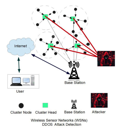
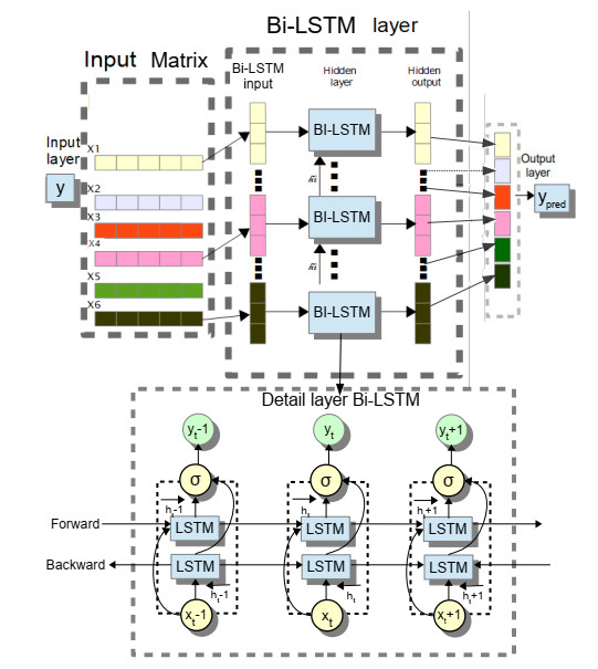
The widespread range of wireless sensor networks (WSNs) has recently increased the possibility of attacks. In the cyber-physical system, WSN is considered a significant component, consisting of several hops that self-organize from moving or stationary sensors. Attackers perform abusive operations to enter, seize, and control the WSN network. In order to stop such attacks on sensor networks in the future, the network traffic data was evaluated, dangerous traffic activity was monitored, and nodes were investigated. In this study, we proposed a new improved bidirectional long-short-term memory (Bi-LSTM) algorithm, which is an enhancement of the LSTM model, to address the issue of intrusion detection in WSN systems, which has four steps. In a preprocessing step, the initial raw data collected from the network can be used to train learning models. Then, the analyzed data was classified according to the types of network traffic, and the attacks were detected in the second step. In the next step, our proposed improved learning models showed results with higher accuracy than traditional detection methods. This study assessed the performance of deep learning algorithms on two different datasets, primarily the 'WSN-DS' and 'KDDCup99' datasets, which were chosen to identify and classify different DoS attacks. The primary common WSN attacks were flooding, scheduling, blackhole, and grayhole, which were included in the data set 'WSN-DS', and (denial-of-service (DoS), user-2-root (U2R), root-2-local (R2L), and Probe) were in the 'KDDCup99' dataset. Our newly improved proposed model based on Bi-LSTM achieved an accuracy of 100% on the 'WSN-DS' dataset and 99.9% on the 'KDDCup99' dataset.
Citation: Ra'ed M. Al-Khatib, Laila Heilat, Wala Qudah, Salem Alhatamleh, Asef Al-Khateeb. A novel improved deep learning model based on Bi-LSTM algorithm for intrusion detection in WSN[J]. Networks and Heterogeneous Media, 2025, 20(2): 532-565. doi: 10.3934/nhm.2025024
The widespread range of wireless sensor networks (WSNs) has recently increased the possibility of attacks. In the cyber-physical system, WSN is considered a significant component, consisting of several hops that self-organize from moving or stationary sensors. Attackers perform abusive operations to enter, seize, and control the WSN network. In order to stop such attacks on sensor networks in the future, the network traffic data was evaluated, dangerous traffic activity was monitored, and nodes were investigated. In this study, we proposed a new improved bidirectional long-short-term memory (Bi-LSTM) algorithm, which is an enhancement of the LSTM model, to address the issue of intrusion detection in WSN systems, which has four steps. In a preprocessing step, the initial raw data collected from the network can be used to train learning models. Then, the analyzed data was classified according to the types of network traffic, and the attacks were detected in the second step. In the next step, our proposed improved learning models showed results with higher accuracy than traditional detection methods. This study assessed the performance of deep learning algorithms on two different datasets, primarily the 'WSN-DS' and 'KDDCup99' datasets, which were chosen to identify and classify different DoS attacks. The primary common WSN attacks were flooding, scheduling, blackhole, and grayhole, which were included in the data set 'WSN-DS', and (denial-of-service (DoS), user-2-root (U2R), root-2-local (R2L), and Probe) were in the 'KDDCup99' dataset. Our newly improved proposed model based on Bi-LSTM achieved an accuracy of 100% on the 'WSN-DS' dataset and 99.9% on the 'KDDCup99' dataset.

| [1] |
I. Almomani, B. Al-Kasasbeh, M. Al-Akhras, Wsn-DS: A dataset for intrusion detection systems in wireless sensor networks, J. Sens., 2016 (2016), 4731953. https://doi.org/10.1155/2016/4731953 doi: 10.1155/2016/4731953

|
| [2] |
K. M. Nahar, R. M. Al-Khatib, M. Barhoush, A. A. Halin, Mpf-leach: Modified probability function for cluster head election in leach protocol, Int. J. Comput. Appl. Technol., 60 (2019), 267–280. https://doi.org/10.1504/IJCAT.2019.100295 doi: 10.1504/IJCAT.2019.100295
|
| [3] | D. Hemanand, G. V. Reddy, S. S. Babu, K. R. Balmuri, T. Chitra, S. Gopalakrishnan, An intelligent intrusion detection and classification system using csgo-lsvm model for wireless sensor networks (WSNs), Int. J. Intell. Syst. Appl. Eng., 10 (2022), 285–293. |
| [4] | M. S. Alsahli, M. M. Almasri, M. Al-Akhras, A. I. Al-Issa, M. Alawairdhi, Evaluation of machine learning algorithms for intrusion detection system in WSN, Int. J. Adv. Comput. Sci. Appl., 12 (2021). |
| [5] |
R. M. Al-Khatib, N. E. A. Al-qudah, M. S. Jawarneh, A. Al-Khateeb, A novel improved lemurs optimization algorithm for feature selection problems, J. King Saud. Univ. Comput. Inf. Sci., 35 (2023), 101704. https://doi.org/10.1016/j.jksuci.2023.101704 doi: 10.1016/j.jksuci.2023.101704
|
| [6] |
P. Nancy, S. Muthurajkumar, S. Ganapathy, S. Santhosh Kumar, M. Selvi, K. Arputharaj, Intrusion detection using dynamic feature selection and fuzzy temporal decision tree classification for wireless sensor networks, IET Commun., 14 (2020), 888–895. https://doi.org/10.1049/iet-com.2019.0172 doi: 10.1049/iet-com.2019.0172
|
| [7] | A. Migdady, A. Al-Aiad, R. M. Al-Khatib, Efficientnet deep learning model for pneumothorax disease detection in chest X-rays images, Int. J. Bus. Inf. Syst., 2022. |
| [8] | N. K. Mittal, A survey on wireless sensor network for community intrusion detection systems, in 2016 3rd International Conference on Recent Advances in Information Technology (RAIT), Dhanbad, India, (2016), 107–111. https://doi.org/10.1109/RAIT.2016.7507884 |
| [9] | K. M. Nahar, R. M. Al-Khatib, M. A. Al-Shannaq, M. M. Barhoush, An efficient holy Quran recitation recognizer based on SVM learning model, Jordanian J. Comput. Inf. Technol., 6 (2020), 395–417. |
| [10] |
H. S. Sharma, A. Sarkar, M. M. Singh, An efficient deep learning-based solution for network intrusion detection in wireless sensor network, Int. J. Syst. Assur. Eng. Manage., 14 (2023), 2423–2446. https://doi.org/10.1007/s13198-023-02090-0 doi: 10.1007/s13198-023-02090-0
|
| [11] |
M. Lopez-Martin, A. Sanchez-Esguevillas, J. I. Arribas, B. Carro, Supervised contrastive learning over prototype-label embeddings for network intrusion detection, Inf. Fusion, 79 (2022), 200–228. https://doi.org/10.1016/j.inffus.2021.09.014 doi: 10.1016/j.inffus.2021.09.014
|
| [12] | M. L. Martin, A. Sanchez-Esguevillas, B. Carro, Review of methods to predict connectivity of iot wireless devices, Novel Appl. Mach. Learn. Network Traffic Anal. Prediction, (2017), 95. |
| [13] |
R. M. Al-Khatib, M. A. Al-Betar, M. A. Awadallah, K. M. Nahar, M. M. A. Shquier, A. M. Manasrah, et al., MGA-TSP: Modernised genetic algorithm for the travelling salesman problem, Int. J. Reasoning-based Intell. Syst., 11 (2019), 215–226. https://doi.org/10.1504/IJRIS.2019.102541 doi: 10.1504/IJRIS.2019.102541
|
| [14] |
D. Sarkar, S. Kumar, P. Das, H. Ramos, Higher-order convergence analysis for interior and boundary layers in a semi-linear reaction-diffusion system networked by a $ k $-star graph with non-smooth source terms, Networks Heterogen. Media, 19 (2024), 1085–1115. https://doi.org/10.3934/nhm.2024048 doi: 10.3934/nhm.2024048
|
| [15] | S. Kumar, P. Das, K. Kumar, Adaptive mesh based efficient approximations for darcy scale precipitation-dissolution models in porous media, Int. J. Numer. Methods Fluids, 96 (2024)a, 1415–1444. https://doi.org/10.1002/fld.5294 |
| [16] |
S. Kumar, P. Das, A uniformly convergent analysis for multiple scale parabolic singularly perturbed convection-diffusion coupled systems: Optimal accuracy with less computational time, Appl. Numer. Math., 207 (2025), 534–557. https://doi.org/10.1016/j.apnum.2024.09.020 doi: 10.1016/j.apnum.2024.09.020
|
| [17] |
S. Jiang, J. Zhao, X. Xu, Slgbm: An intrusion detection mechanism for wireless sensor networks in smart environments, IEEE Access, 8 (2020), 169548–169558. 10.1109/ACCESS.2020.3024219 doi: 10.1109/ACCESS.2020.3024219
|
| [18] |
S. Saini, P. Das, S. Kumar, Parameter uniform higher order numerical treatment for singularly perturbed robin type parabolic reaction diffusion multiple scale problems with large delay in time, Appl. Numer. Math., 196 (2024), 1–21. https://doi.org/10.1016/j.apnum.2023.10.003 doi: 10.1016/j.apnum.2023.10.003
|
| [19] |
K. Kumar, P. C. Podila, P. Das, H. Ramos, A graded mesh refinement approach for boundary layer originated singularly perturbed time-delayed parabolic convection diffusion problems, Math. Methods Appl. Sci., 44 (2021), 12332–12350. https://doi.org/10.1002/mma.7358 doi: 10.1002/mma.7358
|
| [20] | M. S. Jawarneh, S. M. Shah, M. M. Aljawarneh, R. M. Al-Khatib, M. G. Al-Bashayreh, Rib bone extraction towards liver isolating in ct scans using active contour segmentation methods, Int. J. Adv. Comput. Sci. Appl., 16 (2025). |
| [21] |
C. Cai, Y. Tao, T. Zhu, Z. Deng, Short-term load forecasting based on deep learning bidirectional lstm neural network, Appl. Sci., 11 (2021), 8129. https://doi.org/10.3390/app11178129 doi: 10.3390/app11178129
|
| [22] |
R. M. Al-Khatib, N. K. T. El-Omari, M. A. Al-Betar, Innovative cloud computing object-oriented model to unify heterogeneous data, Int. J. Oper. Res., 46 (2023), 289–322. https://doi.org/10.1504/IJOR.2023.129410 doi: 10.1504/IJOR.2023.129410
|
| [23] |
N. A. Alrajeh, S. Khan, B. Shams, Intrusion detection systems in wireless sensor networks: A review, Int. J. Distrib. Sens. Netw., 9 (2013), 167575. https://doi.org/10.1155/2013/167575 doi: 10.1155/2013/167575
|
| [24] | W. Lee, S. J. Stolfo, K. W. Mok, Mining in a data-flow environment: Experience in network intrusion detection, in Proceedings of the Fifth ACM SIGKDD International Conference on Knowledge Discovery and Data Mining, (1999), 114–124. |
| [25] | W. Lee, S. J. Stolfo, K. W. Mok, A data mining framework for building intrusion detection models, in Proceedings of the 1999 IEEE Symposium on Security and Privacy (Cat. No. 99CB36344), Oakland, CA, USA, (1999), 120–132. https://doi.org/10.1109/SECPRI.1999.766909 |
| [26] |
M. Dener, C. Okur, S. Al, A. Orman, WSN-BFSF: A new dataset for attacks detection in wireless sensor networks, IEEE Internet Things J., 11 (2023), 2109–2125. https://doi.org/10.1109/JIOT.2023.329220 doi: 10.1109/JIOT.2023.329220
|
| [27] |
S. Salmi, L. Oughdir, Performance evaluation of deep learning techniques for dos attacks detection in wireless sensor network, J. Big Data, 10 (2023), 1–25. https://doi.org/10.1186/s40537-023-00692-w doi: 10.1186/s40537-023-00692-w
|
| [28] | H. S. Sharma, M. M. Singh, A. Sarkar, Machine learning-based dos attack detection techniques in wireless sensor network: A review, in Proceedings of the International Conference on Cognitive and Intelligent Computing: ICCIC 2021, Springer Nature Singapore, Singapore, 2 (2023), 583–591. |
| [29] | B. J. Santhosh, Kddcup99, 2025. Available from: https://ieee-dataport.org/documents/kddcup99#files. |
| [30] |
S. Choudhary, N. Kesswani, Analysis of KDD-Cup'99, NSL-KDD and UNSW-NB15 datasets using deep learning in LoT, Procedia Comput. Sci., 167 (2020), 1561–1573. https://doi.org/10.1016/j.procs.2020.03.367 doi: 10.1016/j.procs.2020.03.367
|
| [31] |
H. Rashaideh, A. Sawaie, M. A. Al-Betar, L. M. Abualigah, M. M. Al-Laham, R. M. Al-Khatib, et al., A grey wolf optimizer for text document clustering, Int. J. Intell. Syst., 29 (2020), 814–830. https://doi.org/10.1515/jisys-2018-0194 doi: 10.1515/jisys-2018-0194
|
| [32] | S. Overflow, Kdd1999 dataset features exolaination, 2025. Available from: https://stackoverflow.com/questions/17024961/kdd1999-dataset-features-exolaination. |
| [33] | K. F, Long-short-term memory (lstmwsn_1), 2023. Available from: https://www.kaggle.com/code/kamalfstudify/lstmwsn-1. |
| [34] |
Q. Abuein, M. Ra'ed, A. Migdady, M. S. Jawarneh, A. Al-Khateeb, Arsa-tweets: A novel arabic sarcasm detection system based on deep learning model, Heliyon, 10 (2024), e36892. https://doi.org/10.1016/j.heliyon.2024.e36892 doi: 10.1016/j.heliyon.2024.e36892
|
| [35] |
P. Das, An a posteriori based convergence analysis for a nonlinear singularly perturbed system of delay differential equations on an adaptive mesh, Numer. Algorithms, 81 (2019), 465–487. https://doi.org/10.1007/s11075-018-0557-4 doi: 10.1007/s11075-018-0557-4
|
| [36] |
K. L. Chiew, B. Hui, An improved network intrusion detection method based on cnn-lstm-sa, J. Adv. Res. Appl. Sci. Eng. Technol., 1 (2025), 225–238. https://doi.org/10.37934/araset.44.1.225238 doi: 10.37934/araset.44.1.225238
|
| [37] | S. Kumar, S. Kumar, P. Das, Second-order a priori and a posteriori error estimations for integral boundary value problems of nonlinear singularly perturbed parameterized form, Numer. Algorithms, (2024)b, 1–28. https://doi.org/10.1007/s11075-024-01918-5 |
| [38] |
S. Kumar, P. Das, Impact of mixed boundary conditions and nonsmooth data on layer-originated nonpremixed combustion problems: Higher-order convergence analysis, Stud. Appl. Math., 153 (2024), e12763. https://doi.org/10.1111/sapm.12763 doi: 10.1111/sapm.12763
|
| [39] |
I. Abu Doush, M. A. Al-Betar, M. A. Awadallah, A. I. Hammouri, R. M. Al-Khatib, S. ElMustafa, et al., Harmony search algorithm for patient admission scheduling problem, Int. J. Intell. Syst., 29 (2019), 540–553. https://doi.org/10.1515/jisys-2018-0094 doi: 10.1515/jisys-2018-0094
|
| [40] | S. Siami-Namini, N. Tavakoli, A. S. Namin, The performance of lstm and bilstm in forecasting time series, in 2019 IEEE International Conference on Big Data (Big Data), (2019), 3285–3292. https://doi.org/10.1109/BigData47090.2019.9005997 |
Figures(15) / Tables(10)
Ra'ed M. Al-Khatib, Laila Heilat, Wala Qudah, Salem Alhatamleh, Asef Al-Khateeb. A novel improved deep learning model based on Bi-LSTM algorithm for intrusion detection in WSN[J]. Networks and Heterogeneous Media, 2025, 20(2): 532-565. doi: 10.3934/nhm.2025024


 DownLoad: