Optimal fractional sliding mode control for the frequency stability of a hybrid industrial microgrid

Dipak R. Swain; Sunita S. Biswal; Pravat Kumar Rout; P. K. Ray; R. K. Jena; Dipak R. Swain; Sunita S. Biswal; Pravat Kumar Rout; P. K. Ray; R. K. Jena

doi:10.3934/electreng.2023002

AIMS Electronics and Electrical Engineering

2023, Volume 7, Issue 1: 14-37. doi: 10.3934/electreng.2023002

Previous Article Next Article

Research article

Optimal fractional sliding mode control for the frequency stability of a hybrid industrial microgrid

1.
Department of Electrical Engineering, Odisha University of Technology and Research, Bhubaneswar, India
2.
Department of Electrical and Electronics Engineering, Siksha 'O' Anusandhan University, Bhubaneswar, India
3.
Department of Electrical Engineering, Centre for Advanced Post Graduate Studies, Rourkela, India

Received: 31 August 2022 Revised: 22 October 2022 Accepted: 04 November 2022 Published: 14 December 2022

The rising proportion of inverter-based renewable energy sources in current power systems has reduced the rotational inertia of overall microgrid systems. This may cause high-frequency fluctuations in the system leading to system instability. Several initiatives have been suggested concerning inertia emulation based on other integrated external energy sources, such as energy storage systems, to combat the ever-declining issue of inertia. Hence, to deal with the aforementioned issue, we suggest the development of an optimal fractional sliding mode control (FSMC)-based frequency stabilization strategy for an industrial hybrid microgrid. An explicit state-space industrial microgrids model comprised of several coordinated energy sources along with loads, storage systems, photovoltaic and wind farms, is considered. In addition to this, the impact of electric vehicles and batteries with adequate control of the state of charge was investigated due to their short regulation times and this helps to balance the power supply and demand that in turn brings the minimization of the frequency deviations. The performance of the FSMC controller is enhanced by setting optimal parameters by employing the tuning strategy based on an iterative teaching-learning-based optimizer (ITLBO). To justify the efficacy of the proposed controller, the simulated results were obtained under several system conditions by using a vehicle simulator in a MATLAB/Simulink environment. The results reveal the enhanced performance of the ITLBO optimized fractional sliding mode control to effectively damp the frequency oscillations and retain the frequency stability with robustness, quick damping, and reliability under different system conditions.
Citation: Dipak R. Swain, Sunita S. Biswal, Pravat Kumar Rout, P. K. Ray, R. K. Jena. Optimal fractional sliding mode control for the frequency stability of a hybrid industrial microgrid[J]. AIMS Electronics and Electrical Engineering, 2023, 7(1): 14-37. doi: 10.3934/electreng.2023002

Related Papers:

Abstract

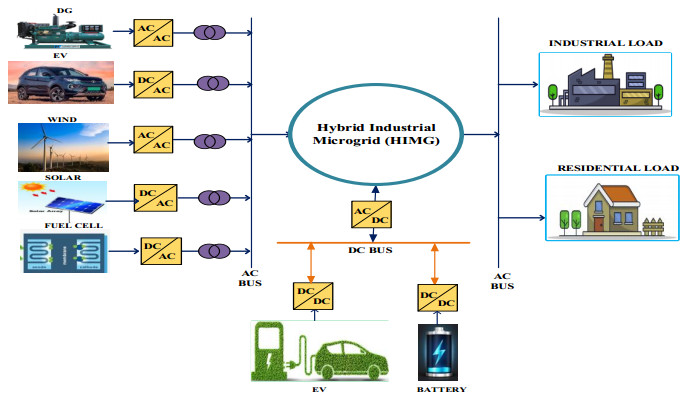
The rising proportion of inverter-based renewable energy sources in current power systems has reduced the rotational inertia of overall microgrid systems. This may cause high-frequency fluctuations in the system leading to system instability. Several initiatives have been suggested concerning inertia emulation based on other integrated external energy sources, such as energy storage systems, to combat the ever-declining issue of inertia. Hence, to deal with the aforementioned issue, we suggest the development of an optimal fractional sliding mode control (FSMC)-based frequency stabilization strategy for an industrial hybrid microgrid. An explicit state-space industrial microgrids model comprised of several coordinated energy sources along with loads, storage systems, photovoltaic and wind farms, is considered. In addition to this, the impact of electric vehicles and batteries with adequate control of the state of charge was investigated due to their short regulation times and this helps to balance the power supply and demand that in turn brings the minimization of the frequency deviations. The performance of the FSMC controller is enhanced by setting optimal parameters by employing the tuning strategy based on an iterative teaching-learning-based optimizer (ITLBO). To justify the efficacy of the proposed controller, the simulated results were obtained under several system conditions by using a vehicle simulator in a MATLAB/Simulink environment. The results reveal the enhanced performance of the ITLBO optimized fractional sliding mode control to effectively damp the frequency oscillations and retain the frequency stability with robustness, quick damping, and reliability under different system conditions.

References

[1]	Davison MJ, Summers TJ, Townsend CD (2017) A review of the distributed generation landscape, key limitations of traditional microgrid concept & possible solution using an enhanced microgrid architecture. 2017 IEEE southern power electronics conference (SPEC), 1-6. IEEE. https://doi.org/10.1109/SPEC.2017.8333563
[2]	Rajesh KS, Dash SS, Rajagopal R, et al. (2017) A review on control of ac microgrid. Renew Sust Energ Rev 71: 814-819. https://doi.org/10.1016/j.rser.2016.12.106 doi: 10.1016/j.rser.2016.12.106
[3]	Shuai Z, Sun Y, Shen ZJ, et al. (2016) Microgrid stability: Classification and a review. Renew Sust Energ Rev 58: 167-179. https://doi.org/10.1016/j.rser.2015.12.201 doi: 10.1016/j.rser.2015.12.201
[4]	Kaur A, Kaushal J, Basak P (2016) A review on microgrid central controller. Renew Sust Energ Rev 55: 338-345. https://doi.org/10.1016/j.rser.2015.10.141 doi: 10.1016/j.rser.2015.10.141
[5]	Barik AK, Jaiswal S, Das DC (2022) Recent trends and development in hybrid microgrid: a review on energy resource planning and control. Int J Sustain Energy 41: 308-322. https://doi.org/10.1080/14786451.2021.1910698 doi: 10.1080/14786451.2021.1910698
[6]	Yakout AH, Kotb H, Hasanien HM, et al. (2021) Optimal fuzzy PIDF load frequency controller for hybrid microgrid system using marine predator algorithm. IEEE Access 9: 54220-54232. https://doi.org/10.1109/ACCESS.2021.3070076 doi: 10.1109/ACCESS.2021.3070076
[7]	Ferrario AM, Bartolini A, Manzano FS, Vivas, et al. (2021) A model-based parametric and optimal sizing of a battery/hydrogen storage of a real hybrid microgrid supplying a residential load: Towards island operation. Advances in Applied Energy 3: 100048. https://doi.org/10.1016/j.adapen.2021.100048 doi: 10.1016/j.adapen.2021.100048
[8]	Kharrich M, Kamel S, Alghamdi AS, et al. (2021) Optimal design of an isolated hybrid microgrid for enhanced deployment of renewable energy sources in Saudi Arabia. Sustainability 13: 4708. https://doi.org/10.3390/su13094708 doi: 10.3390/su13094708
[9]	Ali H, Magdy G, Xu D (2021) A new optimal robust controller for frequency stability of interconnected hybrid microgrids considering non-inertia sources and uncertainties. Int J Elec Power 128: 106651. https://doi.org/10.1016/j.ijepes.2020.106651 doi: 10.1016/j.ijepes.2020.106651
[10]	Gutiérrez-Oliva D, Colmenar-Santos A, Rosales-Asensio E (2022) A Review of the State of the Art of Industrial Microgrids Based on Renewable Energy. Electronics 11: 1002. https://doi.org/10.3390/electronics11071002 doi: 10.3390/electronics11071002
[11]	Yang Q, Li J, Yang R, et al. (2022) New hybrid scheme with local battery energy storages and electric vehicles for the power frequency service. eTransportation 11: 100151. https://doi.org/10.1016/j.etran.2021.100151 doi: 10.1016/j.etran.2021.100151
[12]	Naderi M, Bahramara S, Khayat Y, et al. (2017) Optimal planning in a developing industrial microgrid with sensitive loads. Energy Rep 3: 124-134. https://doi.org/10.1016/j.egyr.2017.08.004 doi: 10.1016/j.egyr.2017.08.004
[13]	Mohamed S, Mokhtar M, Marei MI (2022) An Adaptive Control of Remote Hybrid Microgrid based on the CMPN Algorithm. Electr Pow Syst Res 213: 108793. https://doi.org/10.1016/j.epsr.2022.108793 doi: 10.1016/j.epsr.2022.108793
[14]	Scheubel C, Zipperle T, Tzscheutschler P (2017) Modeling of industrial-scale hybrid renewable energy systems (HRES)–The profitability of decentralized supply for industry. Renew Energ 108: 52-63. https://doi.org/10.1016/j.renene.2017.02.038 doi: 10.1016/j.renene.2017.02.038
[15]	Gamarra C, Guerrero JM, Montero E (2016) A knowledge discovery in databases approach for industrial microgrid planning. Renew Sust Energ Rev 60: 615-630. https://doi.org/10.1016/j.rser.2016.01.091 doi: 10.1016/j.rser.2016.01.091
[16]	Lu R, Bai R, Ding Y, et al. (2021) A hybrid deep learning-based online energy management scheme for industrial microgrid. Appl Energ 304: 117857. https://doi.org/10.1016/j.apenergy.2021.117857 doi: 10.1016/j.apenergy.2021.117857
[17]	Sedaghati R, Shakarami MR (2019) A novel control strategy and power management of hybrid PV/FC/SC/battery renewable power system-based grid-connected microgrid. Sustain Cities Soc 44: 830-843. https://doi.org/10.1016/j.scs.2018.11.014 doi: 10.1016/j.scs.2018.11.014
[18]	Teimourzadeh Baboli P, Shahparasti M, Parsa Moghaddam M, et al. (2014) Energy management and operation modelling of hybrid AC–DC microgrid. IET Gener Transm Dis 8: 1700-1711. https://doi.org/10.1049/iet-gtd.2013.0793 doi: 10.1049/iet-gtd.2013.0793
[19]	Khooban MH, Niknam T, Shasadeghi M, et al. (2017) Load frequency control in microgrids based on a stochastic noninteger controller. IEEE T Sustain Energ 9: 853-861. https://doi.org/10.1109/TSTE.2017.2763607 doi: 10.1109/TSTE.2017.2763607
[20]	Magdy G, Ali H, Xu D (2021) Effective control of smart hybrid power systems: Cooperation of robust LFC and virtual inertia control system. CSEE Journal of Power and Energy Systems.
[21]	Veronica AJ, Kumar NS (2017) Development of hybrid microgrid model for frequency stabilization. Wind Eng 41: 343-352. https://doi.org/10.1177/0309524X17723203 doi: 10.1177/0309524X17723203
[22]	Jampeethong P, Khomfoi S (2020) Coordinated control of electric vehicles and renewable energy sources for frequency regulation in microgrids. IEEE Access 8: 141967-141976. https://doi.org/10.1109/ACCESS.2020.3010276 doi: 10.1109/ACCESS.2020.3010276
[23]	Khokhar B, Dahiya S, Singh Parmar KP (2020) A robust cascade controller for load frequency control of a standalone microgrid incorporating electric vehicles. Electr Pow Compo Sys 48: 711-726. https://doi.org/10.1080/15325008.2020.1797936 doi: 10.1080/15325008.2020.1797936
[24]	Sabhahit JN, Solanke SS, Jadoun VK, et al. (2022) Contingency Analysis of a Grid of Connected EVs for Primary Frequency Control of an Industrial Microgrid Using Efficient Control Scheme. Energies 15: 3102. https://doi.org/10.3390/en15093102 doi: 10.3390/en15093102
[25]	Baghaee HR, Mirsalim M, Gharehpetian GB, et al. (2017) Decentralized sliding mode control of WG/PV/FC microgrids under unbalanced and nonlinear load conditions for on-and off-grid modes. IEEE Syst J 12: 3108-3119. https://doi.org/10.1109/JSYST.2017.2761792 doi: 10.1109/JSYST.2017.2761792
[26]	Khokhar B, Parmar KS (2022) A novel adaptive intelligent MPC scheme for frequency stabilization of a microgrid considering SoC control of EVs. Appl Energ 309: 118423. https://doi.org/10.1016/j.apenergy.2021.118423 doi: 10.1016/j.apenergy.2021.118423
[27]	Dechanupaprittha S, Jamroen C (2021) Self-learning PSO based optimal EVs charging power control strategy for frequency stabilization considering frequency deviation and impact on EV owner. Sustain Energy Grids 26: 100463. https://doi.org/10.1016/j.segan.2021.100463 doi: 10.1016/j.segan.2021.100463
[28]	Hatahet W, Marei MI, Mokhtar M (2021) Adaptive controllers for grid-connected DC microgrids. Int J Elec Power 130: 106917. https://doi.org/10.1016/j.ijepes.2021.106917 doi: 10.1016/j.ijepes.2021.106917
[29]	Ahmed T, Waqar A, Elavarasan RM, et al. (2021) Analysis of fractional order sliding mode control in a d-statcom integrated power distribution system. IEEE Access 9: 70337-70352. https://doi.org/10.1109/ACCESS.2021.3078608 doi: 10.1109/ACCESS.2021.3078608
[30]	Esfahani Z, Roohi M, Gheisarnejad M, et al. (2019) Optimal non-integer sliding mode control for frequency regulation in stand-alone modern power grids. Applied Sciences 9: 3411. https://doi.org/10.3390/app9163411 doi: 10.3390/app9163411
[31]	Aryan Nezhad M, Bevrani H (2018) Frequency control in an islanded hybrid microgrid using frequency response analysis tools. IET Renew Power Gen 12: 227-243. https://doi.org/10.1049/iet-rpg.2017.0227 doi: 10.1049/iet-rpg.2017.0227
[32]	Gorripotu TS, Samalla H, Rao JM, et al. (2019) TLBO algorithm optimized fractional-order PID controller for AGC of interconnected power system. Soft computing in data analytics, 847-855. Springer, Singapore. https: //doi.org/10.1007/978-981-13-0514-6_80
[33]	Bouchekara HREH, Javaid MS, Shaaban YA, et al. (2021) Decomposition based multiobjective evolutionary algorithm for PV/Wind/Diesel Hybrid Microgrid System design considering load uncertainty. Energy Rep 7: 52-69. https://doi.org/10.1016/j.egyr.2020.11.102 doi: 10.1016/j.egyr.2020.11.102
[34]	Bihari SP, Sadhu PK, Sarita K, et al. (2021) A comprehensive review of microgrid control mechanism and impact assessment for hybrid renewable energy integration. IEEE Access.
[35]	Vachirasricirikul S, Ngamroo I (2012) Robust controller design of microturbine and electrolyzer for frequency stabilization in a microgrid system with plug-in hybrid electric vehicles. Int J Elec Power 43: 804-811. https://doi.org/10.1016/j.ijepes.2012.06.029 doi: 10.1016/j.ijepes.2012.06.029
[36]	Khooban MH (2017) Secondary load frequency control of time-delay stand-alone microgrids with electric vehicles. IEEE T Ind Electron 65: 7416-7422. https://doi.org/10.1109/TIE.2017.2784385 doi: 10.1109/TIE.2017.2784385
[37]	Rahman MS, Hossain MJ, Lu J, et al. (2019) A vehicle-to-microgrid framework with optimization-incorporated distributed EV coordination for a commercial neighborhood. IEEE T Ind Inform 16: 1788-1798. https://doi.org/10.1109/TⅡ.2019.2924707 doi: 10.1109/TⅡ.2019.2924707
[38]	Zhu X, Xia M, Chiang HD (2018) Coordinated sectional droop charging control for EV aggregator enhancing frequency stability of microgrid with high penetration of renewable energy sources. Appl Energ 210: 936-943. https://doi.org/10.1016/j.apenergy.2017.07.087 doi: 10.1016/j.apenergy.2017.07.087
[39]	ur Rehman U (2022) A robust vehicle to grid aggregation framework for electric vehicles charging cost minimization and for smart grid regulation. Int J Elec Power 140: 108090. https://doi.org/10.1016/j.ijepes.2022.108090 doi: 10.1016/j.ijepes.2022.108090
[40]	Zaihidee FM, Mekhilef S, Mubin M (2019) Application of fractional order sliding mode control for speed control of permanent magnet synchronous motor. IEEE Access 7: 101765-101774. https://doi.org/10.1109/ACCESS.2019.2931324 doi: 10.1109/ACCESS.2019.2931324
[41]	Li C, Deng W (2007) Remarks on fractional derivatives. Appl Math Comput 187: 777-784. https://doi.org/10.1016/j.amc.2006.08.163 doi: 10.1016/j.amc.2006.08.163
[42]	Li Y, Chen Y, Podlubny I (2010) Stability of fractional-order nonlinear dynamic systems: Lyapunov direct method and generalized Mittag–Leffler stability. Comput Math Appl 59: 1810-1821. https://doi.org/10.1016/j.camwa.2009.08.019 doi: 10.1016/j.camwa.2009.08.019
[43]	Rao Venkata R (2015) Teaching-learning-based optimization algorithm. Teaching learning based optimization algorithm, 9-39. https://doi.org/10.1007/978-3-319-22732-0_2.
[44]	Biswal, S. S., Swain, D. R., & Rout, P. K. (2021, October). VSC based HVDC Transmission System using Adaptive FPI Controller. In 2021 International Conference in Advances in Power, Signal, and Information Technology (APSIT) (pp. 1-6). IEEE.
[45]	Yang B, Yu T, Zhang X, et al. (2018) Interactive teaching–learning optimiser for parameter tuning of VSC-HVDC systems with offshore wind farm integration. IET Gener Transm Dis 12: 678-687. https://doi.org/10.1049/iet-gtd.2016.1768 doi: 10.1049/iet-gtd.2016.1768

Reader Comments

Your name:*

Email:*
© 2023 the Author(s), licensee AIMS Press. This is an open access article distributed under the terms of the Creative Commons Attribution License (http://creativecommons.org/licenses/by/4.0)