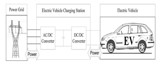
Electric vehicles (EVs) are an emerging technology that contribute to reducing air pollution. This paper presents the development of a 200 kW DC charger for the vehicle-to-grid (V2G) application. The bidirectional dual active bridge (DAB) converter was the preferred fit for a high-power DC-DC conversion due its attractive features such as high power density and bidirectional power flow. A particle swarm optimization (PSO) algorithm was used to online auto-tune the optimal proportional gain (KP) and integral gain (KI) value with minimized error voltage. Then, knowing that the controller with fixed gains have limitation in its response during dynamic change, the PSO was improved to allow re-tuning and update the new KP and KI upon step changes or disturbances through a time-variant approach. The proposed controller, online auto-tuned PI using PSO with re-tuning (OPSO-PI-RT) and one-time (OPSO-PI-OT) execution were compared under desired output voltage step changes and load step changes in terms of steady-state error and dynamic performance. The OPSO-PI-RT method was a superior controller with 98.16% accuracy and faster controller with 85.28 s-1 average speed compared to OPSO-PI-OT using controller hardware-in-the-loop (CHIL) approach.
Citation: Suliana Ab-Ghani, Hamdan Daniyal, Abu Zaharin Ahmad, Norazila Jaalam, Norhafidzah Mohd Saad, Nur Huda Ramlan, Norhazilina Bahari. Adaptive online auto-tuning using Particle Swarm optimized PI controller with time-variant approach for high accuracy and speed in Dual Active Bridge converter[J]. AIMS Electronics and Electrical Engineering, 2023, 7(2): 156-170. doi: 10.3934/electreng.2023009
Electric vehicles (EVs) are an emerging technology that contribute to reducing air pollution. This paper presents the development of a 200 kW DC charger for the vehicle-to-grid (V2G) application. The bidirectional dual active bridge (DAB) converter was the preferred fit for a high-power DC-DC conversion due its attractive features such as high power density and bidirectional power flow. A particle swarm optimization (PSO) algorithm was used to online auto-tune the optimal proportional gain (KP) and integral gain (KI) value with minimized error voltage. Then, knowing that the controller with fixed gains have limitation in its response during dynamic change, the PSO was improved to allow re-tuning and update the new KP and KI upon step changes or disturbances through a time-variant approach. The proposed controller, online auto-tuned PI using PSO with re-tuning (OPSO-PI-RT) and one-time (OPSO-PI-OT) execution were compared under desired output voltage step changes and load step changes in terms of steady-state error and dynamic performance. The OPSO-PI-RT method was a superior controller with 98.16% accuracy and faster controller with 85.28 s-1 average speed compared to OPSO-PI-OT using controller hardware-in-the-loop (CHIL) approach.

| [1] |
Bose BK (2010) Global warming: Energy, Environmental Pollution, and the Impact of Power Electronics. IEEE Ind Electron Mag 4: 6–17. https://doi.org/10.1109/MIE.2010.935860 doi: 10.1109/MIE.2010.935860

|
| [2] |
Khan SA, Islam R, Guo Y, Zhu J (2019) A New Isolated Multi-Port Converter With Multi-Directional Power Flow Capabilities for Smart Electric Vehicle Charging Stations. IEEE T Appl Supercon 29: 1–4. https://doi.org/10.1109/TASC.2019.2895526 doi: 10.1109/TASC.2019.2895526
|
| [3] |
Latifi M, Rastegarnia A, Khalili A, Sane S (2018) Agent-Based Decentralized Optimal Charging Strategy for Plug-in Electric Vehicles. IEEE T Ind Electron 66: 3668–3680. https://doi.org/10.1109/TIE.2018.2853609 doi: 10.1109/TIE.2018.2853609
|
| [4] |
Richardson DB (2013) Electric vehicles and the electric grid : A review of modeling approaches, Impacts, and renewable energy integration. Renew Sustain Energy Rev 19: 247–254. https://doi.org/10.1016/j.rser.2012.11.042 doi: 10.1016/j.rser.2012.11.042
|
| [5] |
Rubino L, Capasso C, Veneri O (2017) Review on plug-in electric vehicle charging architectures integrated with distributed energy sources for sustainable mobility. Appl Energy 207: 438–464. https://doi.org/10.1016/j.apenergy.2017.06.097 doi: 10.1016/j.apenergy.2017.06.097
|
| [6] |
Ashique RH, Salam Z, Aziz MJ, Bhatti AR (2017) Integrated photovoltaic-grid dc fast charging system for electric vehicle : A review of the architecture and control. Renew Sustain Energy Rev 69: 1243–1257. https://doi.org/10.1016/j.rser.2016.11.245 doi: 10.1016/j.rser.2016.11.245
|
| [7] | Blech T (2019) CHAdeMO DC charging standard: evolution strategy and new challenges. |
| [8] |
Tan KM, Ramachandaramurthy VK, Yong JY (2016) Integration of electric vehicles in smart grid : A review on vehicle to grid technologies and optimization techniques. Renew Sustain Energy Rev 53: 720–732. https://doi.org/10.1016/j.rser.2015.09.012 doi: 10.1016/j.rser.2015.09.012
|
| [9] |
Sha D, Wang X, Chen D (2017) High-Efficiency Current-Fed Dual Active Bridge DC – DC Converter With ZVS Achievement Throughout Full Range of Load Using Optimized Switching Patterns. IEEE T Power Electron 33: 1347–1357. https://doi.org/10.1109/TPEL.2017.2675945 doi: 10.1109/TPEL.2017.2675945
|
| [10] |
Oggier GG, Garcia GO, Oliva AR (2009) Switching Control Strategy to Minimize Dual Active Bridge Converter Losses. IEEE T Power Electron 24: 1826–1838. https://doi.org/10.1109/TPEL.2009.2020902 doi: 10.1109/TPEL.2009.2020902
|
| [11] |
Waltrich G, Hendrix MA, Duarte JL (2015) Three-Phase Bidirectional DC / DC Converter With Six Inverter Legs in Parallel for EV Applications. IEEE T Ind Electron 63: 1372–1384. https://doi.org/10.1109/TIE.2015.2494001 doi: 10.1109/TIE.2015.2494001
|
| [12] |
Karthikeyan V, Gupta R (2017) Light-load efficiency improvement by extending ZVS range in DAB- bidirectional DC-DC converter for energy storage applications. Energy 130: 15–21. https://doi.org/10.1016/j.energy.2017.04.119 doi: 10.1016/j.energy.2017.04.119
|
| [13] |
De Doncker RW, Divan DM, Kheraluwala MH (1991) A Three-phase Soft-Switched High-Power-Density DC/DC Converter for High Power Applications. IEEE T Ind Appl 27: 63–73. https://doi.org/10.1109/28.67533 doi: 10.1109/28.67533
|
| [14] |
Zhang K, Shan Z, Jatskevich J (2017) Large- and Small-Signal Average-Value Modeling of Dual-Active-Bridge DC-DC Converter Considering Power Losses. IEEE T Power Electron 32: 1964–1974. https://doi.org/10.1109/TPEL.2016.2555929 doi: 10.1109/TPEL.2016.2555929
|
| [15] |
Park Y, Chakraborty S, Khaligh A (2022) DAB Converter for EV Onboard Chargers Using Bare-Die SiC MOSFETs and Leakage-Integrated Planar Transformer. IEEE T Transp Electr 8: 209–224. https://doi.org/10.1109/TTE.2021.3121172 doi: 10.1109/TTE.2021.3121172
|
| [16] |
Li L, Xu G, Xiong W, Liu D, Su M (2021) An Optimized DPS Control for Dual-Active-Bridge Converters to Secure Full-Load-Range ZVS With Low Current Stress. IEEE T Transp Electr 8: 1389–1400. https://doi.org/10.1109/TTE.2021.3106130 doi: 10.1109/TTE.2021.3106130
|
| [17] |
Deželak K, Bracinik P, Sredenšek K, Seme S (2021) Proportional-integral controllers performance of a grid-connected solar pv system with particle swarm optimization and ziegler–nichols tuning method. Energies 14: 2516. https://doi.org/10.3390/en14092516 doi: 10.3390/en14092516
|
| [18] |
Faisal SF, Beig AR, Thomas S (2020) Time Domain Particle Swarm Optimization of PI Controllers for Bidirectional VSC HVDC Light System. Energies 13: 866. https://doi.org/10.3390/en13040866 doi: 10.3390/en13040866
|
| [19] |
Hou N, Song W, Wu M (2016) Minimum-Current-Stress Scheme of Dual Active Bridge DC-DC Converter With Unified Phase-Shift Control. IEEE T Power Electron 31: 8552–8561. https://doi.org/10.1109/TPEL.2016.2521410 doi: 10.1109/TPEL.2016.2521410
|
| [20] |
Shi H, Wen H, Chen J, Hu Y, Jiang L, Chen G, et al. (2018) Minimum-Backflow-Power Scheme of DAB-Based Solid-State Transformer With Extended-Phase-Shift Control. IEEE T Ind Appl 54: 3483–3496. https://doi.org/10.1109/TIA.2018.2819120 doi: 10.1109/TIA.2018.2819120
|
| [21] |
Shi H, Wen H, Hu Y, Jiang L (2018) Reactive Power Minimization in Bidirectional DC – DC Converters Using a Unified-Phasor-Based Particle Swarm Optimization. IEEE T Power Electron 33: 10990–11006. https://doi.org/10.1109/TPEL.2018.2811711 doi: 10.1109/TPEL.2018.2811711
|
| [22] |
Hebala OM, Aboushady AA, Ahmed KH, Abdelsalam I (2018) Generic Closed Loop Controller for Power Regulation in Dual Active Bridge DC / DC Converter with Current Stress Minimization. IEEE T Ind Electron 66: 4468–4478. https://doi.org/10.1109/TIE.2018.2860535 doi: 10.1109/TIE.2018.2860535
|
| [23] |
Hassan M, Ge X, Woldegiorgis AT, Mastoi MS, Shahid MB, Atif R, et al. (2023) A look-up table-based model predictive torque control of IPMSM drives with duty cycle optimization. ISA T. https://doi.org/10.1016/j.isatra.2023.02.007 doi: 10.1016/j.isatra.2023.02.007
|
| [24] |
Xiong F, Wu J, Hao L, Liu Z (2017) Backflow Power Optimization Control for Dual Active Bridge DC-DC Converters. Energies 10: 1–27. https://doi.org/10.3390/en10091403 doi: 10.3390/en10091403
|
| [25] |
Tong A, Hang L, Li G, Jiang X, Gao S (2017) Modeling and Analysis of a DualActive-Bridge-Isolated Bidirectional DC/DC Converter to Minimize RMS Current With Whole Operating Range. IEEE T Power Electron 33: 5302–5316. https://doi.org/10.1109/TPEL.2017.2692276 doi: 10.1109/TPEL.2017.2692276
|
| [26] |
Jaalam N, Ahmad AZ, Khalid AM, Abdullah R, Saad NM, Ghani SA, et al. (2022) Low Voltage Ride through Enhancement Using Grey Wolf Optimizer to Reduce Overshoot Current in the Grid-Connected PV System. Math Probl Eng 2022: 3917775. https://doi.org/10.1155/2022/3917775 doi: 10.1155/2022/3917775
|
| [27] |
Salman SS, Humod AT, Hasan FA (2022) Optimum control for dynamic voltage restorer based on particle swarm optimization algorithm. Indonesian Journal of Electrical Engineering and Computer Science 26: 1351–1359. https://doi.org/10.11591/ijeecs.v26.i3.pp1351-1359 doi: 10.11591/ijeecs.v26.i3.pp1351-1359
|
| [28] |
Kumar R, Bansal HO, Gautam AR, Mahela OP, Khan B (2022) Experimental Investigations on Particle Swarm Optimization Based Control Algorithm for Shunt Active Power Filter to Enhance Electric Power Quality. IEEE Access 10: 54878–54890. https://doi.org/10.1109/ACCESS.2022.3176732 doi: 10.1109/ACCESS.2022.3176732
|
| [29] |
Borin LC, Mattos E, Osorio CR, Koch GG, Montagner VF (2019) Robust PID Controllers Optimized by PSO Algorithm for Power Converters. 2019 IEEE 15th Brazilian Power Electronics Conference and 5th IEEE Southern Power Electronics Conference, COBEP/SPEC, 1‒6. https://doi.org/10.1109/COBEP/SPEC44138.2019.9065642 doi: 10.1109/COBEP/SPEC44138.2019.9065642
|
| [30] |
Song W, Hou N, Wu M (2017) Virtual Direct Power Control Scheme of Dual Active Bridge DC – DC Converters for Fast Dynamic Response. IEEE T Power Electron 33: 1750–1759. https://doi.org/10.1109/TPEL.2017.2682982 doi: 10.1109/TPEL.2017.2682982
|
| [31] |
Hassan M, Ge X, Atif R, Woldegiorgis AT, Mastoi MS, Shahid MB (2022) Computational efficient model predictive current control for interior permanent magnet synchronous motor drives. IET Power Electron 15: 1111–1133. https://doi.org/10.1049/pel2.12294 doi: 10.1049/pel2.12294
|
| [32] |
Zeng D, Zheng Y, Luo W, Hu Y, Cui Q, Li Q, et al. (2019) Research on Improved Auto-Tuning of a PID Controller Based on Phase Angle Margin. Energies 12: 1–16. https://doi.org/10.3390/en12091704 doi: 10.3390/en12091704
|
| [33] |
Sun X, Qiu J (2021) A Customized Voltage Control Strategy for Electric Vehicles in Distribution Networks with Reinforcement Learning Method. IEEE T Ind Inform 17: 6852–6863. https://doi.org/10.1109/TII.2021.3050039 doi: 10.1109/TII.2021.3050039
|
| [34] |
Wang Y, Qiu D, Strbac G, Gao Z (2023) Coordinated Electric Vehicle Active and Reactive Power Control for Active Distribution Networks. IEEE T Ind Inform 19: 1611–1622. https://doi.org/10.1109/TII.2022.3169975 doi: 10.1109/TII.2022.3169975
|
| [35] |
Ab-Ghani S, Daniyal H, Jaalam N, Ramlan NH, Saad NM (2022) Time-Variant Online Auto-Tuned PI Controller Using PSO Algorithm for High Accuracy Dual Active Bridge DC-DC Converter. 2022 IEEE International Conference on Automatic Control and Intelligent Systems, I2CACIS, 36‒41. https://doi.org/10.1109/I2CACIS54679.2022.9815470 doi: 10.1109/I2CACIS54679.2022.9815470
|
| [36] |
Liu H, Song Q, Zhang C, Chen J, Deng B, Li J (2019) Development of bi-directional DC / DC converter for fuel cell hybrid vehicle. J Renew Sustain Energy 11: 44303. https://doi.org/10.1063/1.5094512 doi: 10.1063/1.5094512
|
| [37] |
Yang J, Liu J, Zhang J, Zhao N, Wang Y, Zheng TQ (2018) Multirate Digital Signal Processing and Noise Suppression for Dual Active Bridge DC DC Converters in a Power Electronic Traction Transformer. IEEE T Power Electron 33: 10885–10902. https://doi.org/10.1109/TPEL.2018.2803744 doi: 10.1109/TPEL.2018.2803744
|
| [38] |
Rodriquez A, Vazquez A, Lamar DG, Hernando MM, Sebastia J (2014) Different Purpose Design Strategies and Techniques to Improve the Performance of a Dual Active Bridge With Phase-Shift Control. IEEE T Power Electron 30: 790–804. https://doi.org/10.1109/TPEL.2014.2309853 doi: 10.1109/TPEL.2014.2309853
|
| [39] | Kennedy J, Eberhart R (1995) Particle Swarm Optimization. Proc IEEE Int Conf Neural Networks 4: 1942–1948. |
| [40] |
Ishaque K, Salam Z, Shamsudin A, Amjad M (2012) A direct control based maximum power point tracking method for photovoltaic system under partial shading conditions using particle swarm optimization algorithm. Appl Energy 99: 414–422. https://doi.org/10.1016/j.apenergy.2012.05.026 doi: 10.1016/j.apenergy.2012.05.026
|
| [41] |
Ishaque K, Salam Z, Amjad M, Mekhilef S (2012) An Improved Particle Swarm Optimization (PSO)– Based MPPT for PV With Reduced Steady-State Oscillation. IEEE T Power Electron 27: 3627–3638. https://doi.org/10.1109/TPEL.2012.2185713 doi: 10.1109/TPEL.2012.2185713
|


Figures(13) / Tables(2)

Suliana Ab-Ghani, Hamdan Daniyal, Abu Zaharin Ahmad, Norazila Jaalam, Norhafidzah Mohd Saad, Nur Huda Ramlan, Norhazilina Bahari. Adaptive online auto-tuning using Particle Swarm optimized PI controller with time-variant approach for high accuracy and speed in Dual Active Bridge converter[J]. AIMS Electronics and Electrical Engineering, 2023, 7(2): 156-170. doi: 10.3934/electreng.2023009


 DownLoad: