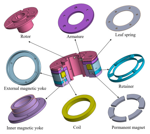
Permanent magnet brake (PMB) is a safe and effective braking mechanism used to stop and hold the load in place. Due to its complex structure and high reliability, assessing the reliability of PMB remains a challenge. The main difficulty lies in that there are several performance indicators reflecting the health state of PMB, and they are correlated with each other. In order to assess the reliability of PMB more accurately, a constant stress accelerated degradation test (ADT) is carried out to collect degradation data of two main performance indicators in PMB. An accelerated bivariate Wiener degradation model is proposed to analyse the ADT data. In the proposed model, the relationship between degradation rate and stress levels is described by Arrhenius model, and a common random effect is introduced to describe the unit-to-unit variation and correlation between the two performance indicators. The Markov Chain Monte Carlo (MCMC) algorithm is performed to obtain the point and interval estimates of the model parameters. Finally, the proposed model and method are applied to analyse the accelerated degradation data of PMB, and the results show that the reliability of PMB at the used condition can be quantified quite well.
Citation: Jihong Pang, Chaohui Zhang, Xinze Lian, Yichao Wu. Reliability assessment of permanent magnet brake based on accelerated bivariate Wiener degradation process[J]. Mathematical Biosciences and Engineering, 2023, 20(7): 12320-12340. doi: 10.3934/mbe.2023548
Permanent magnet brake (PMB) is a safe and effective braking mechanism used to stop and hold the load in place. Due to its complex structure and high reliability, assessing the reliability of PMB remains a challenge. The main difficulty lies in that there are several performance indicators reflecting the health state of PMB, and they are correlated with each other. In order to assess the reliability of PMB more accurately, a constant stress accelerated degradation test (ADT) is carried out to collect degradation data of two main performance indicators in PMB. An accelerated bivariate Wiener degradation model is proposed to analyse the ADT data. In the proposed model, the relationship between degradation rate and stress levels is described by Arrhenius model, and a common random effect is introduced to describe the unit-to-unit variation and correlation between the two performance indicators. The Markov Chain Monte Carlo (MCMC) algorithm is performed to obtain the point and interval estimates of the model parameters. Finally, the proposed model and method are applied to analyse the accelerated degradation data of PMB, and the results show that the reliability of PMB at the used condition can be quantified quite well.

| [1] | Q. Yue, H. Qian, High torque density permanent magnet brake, in 2021 4th International Conference on Mechanical, Electrical and Material Application, 2125 (2021), 012068. https://doi.org/10.1088/1742-6596/2125/1/012068 |
| [2] |
L. Zhuang, A. Xu, X. Wang, A prognostic driven predictive maintenance framework based on Bayesian deep learning, Reliab. Eng. Syst. Saf., 234 (2023), 109181. https://doi.org/10.1016/j.ress.2023.109181 doi: 10.1016/j.ress.2023.109181

|
| [3] |
C. Luo, L. Shen, A. Xu, Modelling and estimation of system reliability under dynamic operating environments and lifetime ordering constraints, Reliab. Eng. Syst. Saf., 218 (2022), 108136. https://doi.org/10.1016/j.ress.2021.108136 doi: 10.1016/j.ress.2021.108136
|
| [4] |
P. Jiang, B. Wang, X. Wang, Z. Zhou, Inverse Gaussian process based reliability analysis for constant-stress accelerated degradation data, Appl. Math. Modell., 105 (2022), 137–148. https://doi.org/10.1016/j.apm.2021.12.003 doi: 10.1016/j.apm.2021.12.003
|
| [5] |
S. Li, Z. Chen, Q. Liu, W. Shi, K. Li, Modeling and analysis of performance degradation data for reliability assessment: A review, IEEE Access, 8 (2020), 74648–74678. https://doi.org/10.1109/ACCESS.2020.2987332 doi: 10.1109/ACCESS.2020.2987332
|
| [6] |
S. Limon, O. P. Yadav, H. Liao, A literature review on planning and analysis of accelerated testing for reliability assessment, Qual. Reliab. Eng. Int., 33 (2017), 2361–2383. https://doi.org/10.1002/qre.2195 doi: 10.1002/qre.2195
|
| [7] |
X. Yuan, E. Higo, M. D. Pandey, Estimation of the value of an inspection and maintenance program: A Bayesian gamma process model, Reliab. Eng. Syst. Saf., 216 (2021), 107912. https://doi.org/10.1016/j.ress.2021.107912 doi: 10.1016/j.ress.2021.107912
|
| [8] |
F, Zhang, J. Li, H. K. T. Ng, Minimum f-divergence estimation with applications to degradation data analysis, IEEE Trans. Inf. Theory, 68 (2022), 6774–6789. https://doi.org/10.1109/TIT.2022.3169885 doi: 10.1109/TIT.2022.3169885
|
| [9] |
W. Yu, Y. Shao, J. Xu, C. Mechefske, An adaptive and generalized Wiener process model with a recursive filtering algorithm for remaining useful life estimation, Reliab. Eng. Syst. Saf., 217 (2022), 108099. https://doi.org/10.1016/j.ress.2021.108099 doi: 10.1016/j.ress.2021.108099
|
| [10] |
H. Wang, H. Liao, X. Ma, R. Bao, Remaining useful life prediction and optimal maintenance time determination for a single unit using isotonic regression and gamma process model, Reliab. Eng. Syst. Saf., 210 (2021), 107504. https://doi.org/10.1016/j.ress.2021.107504 doi: 10.1016/j.ress.2021.107504
|
| [11] |
Z. Ye, N. Chen, The Inverse Gaussian process as a degradation model, Technometrics, 56 (2014), 302–311. https://doi.org/10.1080/00401706.2013.830074 doi: 10.1080/00401706.2013.830074
|
| [12] |
Z. Zhang, X. Si, C. Hu, Y. Lei, Degradation data analysis and remaining useful life estimation: A review on Wiener-process-based methods, Eur. J. Oper. Res., 271 (2018), 775–796. https://doi.org/10.1016/j.ejor.2018.02.033 doi: 10.1016/j.ejor.2018.02.033
|
| [13] |
G. Liao, H. Yin, M. Chen, Z. Lin, Remaining useful life prediction for multi-phase deteriorating process based on Wiener process, Reliab. Eng. Syst. Saf., 207 (2021), 107361. https://doi.org/10.1016/j.ress.2020.107361 doi: 10.1016/j.ress.2020.107361
|
| [14] |
Y. Hou, Y. Du, Y. Peng, D. Liu, An improved random effects Wiener process accelerated degradation test model for lithium-ion battery, IEEE Trans. Instrum. Meas., 70 (2021), 1–11. https://doi.org/10.1109/TIM.2021.3091457 doi: 10.1109/TIM.2021.3091457
|
| [15] |
Q. Zhai, P. Chen, L. Hong, L. Shen, A random-effects Wiener degradation model based on accelerated failure time, Reliab. Eng. Syst. Saf., 180 (2018), 94–103. https://doi.org/10.1016/j.ress.2018.07.003 doi: 10.1016/j.ress.2018.07.003
|
| [16] |
B. Yan, X. Ma, L. Yang, H. Wang, T. Wu, A novel degradation-rate-volatility related effect Wiener process model with its extension to accelerated ageing data analysis, Reliab. Eng. Syst. Saf., 204 (2020), 107138. https://doi.org/10.1016/j.ress.2020.107138 doi: 10.1016/j.ress.2020.107138
|
| [17] |
X. Ye, Y. Hu, B. Zheng, C. Chen, G. Zhai, A new class of multi-stress acceleration models with interaction effects and its extension to accelerated degradation modelling, Reliab. Eng. Syst. Saf., 228 (2022), 108815. https://doi.org/10.1016/j.ress.2022.108815 doi: 10.1016/j.ress.2022.108815
|
| [18] |
P. Jiang, B. Wang, X. Wang, S. Qin, Optimal plan for Wiener constant-stress accelerated degradation model, Appl. Math. Modell., 84 (2020), 191–201. https://doi.org/10.1016/j.apm.2020.03.036 doi: 10.1016/j.apm.2020.03.036
|
| [19] |
P. Jiang, X. Yang, Reliability inference and remaining useful life prediction for the doubly accelerated degradation model based on Wiener process, AIMS Math., 8 (2023), 7560–7583. https://doi.org/10.3934/math.2023379 doi: 10.3934/math.2023379
|
| [20] |
J. Ma, L. Cai, G. Liao, H. Yin, X. Si, P. Zhang, A multi-phase Wiener process-based degradation model with imperfect maintenance activities, Reliab. Eng. Syst. Saf., 232 (2023), 109075. https://doi.org/10.1016/j.ress.2022.109075 doi: 10.1016/j.ress.2022.109075
|
| [21] |
F. Wang, H. Li, On the use of the maximum entropy method for reliability evaluation involving stochastic process modeling, Struct. Saf., 88 (2021), 102028. https://doi.org/10.1016/j.strusafe.2020.102028 doi: 10.1016/j.strusafe.2020.102028
|
| [22] |
R. Chen, C. Zhang, S. Wang, Y. Qian, Reliability estimation of mechanical seals based on bivariate dependence analysis and considering model uncertainty, Chin. J. Aeronaut., 34 (2021), 554–572. https://doi.org/10.1016/j.cja.2020.12.001 doi: 10.1016/j.cja.2020.12.001
|
| [23] |
W. Peng, Y. Li, Y. Yang, S. Zhu, H. Huang, Bivariate analysis of incomplete degradation observations based on inverse gaussian processes and copulas, IEEE Trans. Reliab., 65 (2016), 624–639. https://doi.org/10.1109/tr.2015.2513038 doi: 10.1109/tr.2015.2513038
|
| [24] |
G. Fang, R. Pan, Y. Hong, Copula-based reliability analysis of degrading systems with dependent failures, Reliab. Eng. Syst. Saf., 193 (2020), 106618. https://doi.org/10.1016/j.ress.2019.106618 doi: 10.1016/j.ress.2019.106618
|
| [25] |
K. Song, L. Cui, A common random effect induced bivariate gamma degradation process with application to remaining useful life prediction, Reliab. Eng. Syst. Saf., 219 (2022), 108200. https://doi.org/10.1016/j.ress.2021.108200 doi: 10.1016/j.ress.2021.108200
|
| [26] |
G. Fang, R. Pan, Y. Wang, Inverse Gaussian processes with correlated random effects for multivariate degradation modeling, Eur. J. Oper. Res., 300 (2022), 1177–1193. https://doi.org/10.1016/j.ejor.2021.10.049 doi: 10.1016/j.ejor.2021.10.049
|
| [27] |
Q. Zhai, Z. Ye, A multivariate stochastic degradation model for dependent performance characteristics, Technometrics, (2023), 1–13. https://doi.org/10.1080/00401706.2022.2157881 doi: 10.1080/00401706.2022.2157881
|
| [28] |
B. Yan, H. Wang, X. Ma, Correlation‐driven multivariate degradation modeling and RUL prediction based on Wiener process model, Qual. Reliab. Eng. Int., (2022). https://doi.org/10.1002/qre.3105 doi: 10.1002/qre.3105
|
| [29] |
S. Zhou, Y. Tang, A. Xu, A generalized Wiener process with dependent degradation rate and volatility and time-varying mean-to-variance ratio, Reliab. Eng. Syst. Saf., 216 (2021), 107895. https://doi.org/10.1016/j.ress.2021.107895 doi: 10.1016/j.ress.2021.107895
|
| [30] |
A. Xu, L. Shen, B. Wang, Y. Tang, On modeling bivariate Wiener degradation process, IEEE Trans. Reliab., 67 (2018), 897–906. https://doi.org/10.1109/TR.2018.2791616 doi: 10.1109/TR.2018.2791616
|
| [31] |
Z. Ye, Y. Wang, K. Tsui, M. Pecht, Degradation data analysis using Wiener processes with measurement errors, IEEE Trans. Reliab., 62 (2013), 772–780. https://doi.org/10.1109/TR.2013.2284733 doi: 10.1109/TR.2013.2284733
|
| [32] |
W. Yan, X. Xu, D. Bigaud, W. Cao, Optimal design of step-stress accelerated degradation tests based on the Tweedie exponential dispersion process, Reliab. Eng. Syst. Saf., 230 (2023), 108917. https://doi.org/10.1016/j.ress.2022.108917 doi: 10.1016/j.ress.2022.108917
|
| [33] |
X. Zhao, B. Liu, Y. Liu, Reliability modeling and analysis of load-sharing systems with continuously degrading components, IEEE Trans. Reliab., 67 (2018), 1096–1110. https://doi.org/10.1109/TR.2018.2846649 doi: 10.1109/TR.2018.2846649
|
| [34] |
W. Peng, S. Zhu, L. Shen, The transformed inverse gaussian process as an age-and state-dependent degradation model, Appl. Math. Modell., 75 (2019), 837–852. https://doi.org/10.1016/j.apm.2019.07.004 doi: 10.1016/j.apm.2019.07.004
|
| [35] |
D. W. Joenssen, J. Vogel, A power study of goodness-of-fit tests for multivariate normality implemented in R, J. Stat. Comput. Simul., 84 (2014), 1055–1078. https://doi.org/10.1080/00949655.2012.739620 doi: 10.1080/00949655.2012.739620
|
| [36] |
S. Brooks, A. Gelman, General methods for monitoring convergence of iterative simulations, J. Comput. Graph. Stat., 7 (1998), 434–455. https://doi.org/10.1080/10618600.1998.10474787 doi: 10.1080/10618600.1998.10474787
|


Figures(13) / Tables(2)

Jihong Pang, Chaohui Zhang, Xinze Lian, Yichao Wu. Reliability assessment of permanent magnet brake based on accelerated bivariate Wiener degradation process[J]. Mathematical Biosciences and Engineering, 2023, 20(7): 12320-12340. doi: 10.3934/mbe.2023548


 DownLoad: