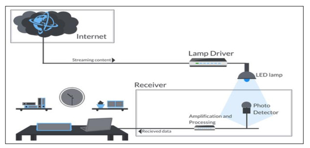
The Internet of Things (IoT) has an ever more significant function in many areas of our modern world. It improves the overall quality of life, where almost everything, including objects and devices, can be linked to the cloud and thus be hyper-connected. Within this changing IoT system, this paper focuses on data transfer, emphasizing the critical role of light fidelity (LiFi) technology. LiFi technology is an up-and-coming technology that makes use of light-emitting diodes (LEDs) and photodetectors (PDs) as transmitters and receivers (RX), respectively, for concurrent data communications and lighting. This paper proposes a single-input multiple-output IoT-based LiFi system using an LED array, phototransistor, and ambient light sensor-based RXS for simultaneous data transmission. DHT11 sensor is used to measure the environmental conditions and store collected data via Wi-Fi in the cloud server using HTTP protocol. Through indoor LiFi communication, the cloud streaming data is transferred using pulse position modulation (PPM) at a frequency of 2 KHz. The experimental results illustrate transferring and receiving data successfully at a communication distance of 1 meter. MATLAB software is used to evaluate the performance of the spatial radiance pattern and illuminance intensity of an LED Array used and received power depending on a line-of-sight (LOS) channel.
Citation: Mostafa A.R. Eltokhy, Mohamed Abdel-Hady, Ayman Haggag, Hisham A. Hamad, Tarek Hosny, Ahmed A. F. Youssef, Ali M. El-Rifaie. An indoor IoT-based LiFi system using LEDs for sensor data transfer[J]. AIMS Electronics and Electrical Engineering, 2025, 9(2): 118-138. doi: 10.3934/electreng.2025007
The Internet of Things (IoT) has an ever more significant function in many areas of our modern world. It improves the overall quality of life, where almost everything, including objects and devices, can be linked to the cloud and thus be hyper-connected. Within this changing IoT system, this paper focuses on data transfer, emphasizing the critical role of light fidelity (LiFi) technology. LiFi technology is an up-and-coming technology that makes use of light-emitting diodes (LEDs) and photodetectors (PDs) as transmitters and receivers (RX), respectively, for concurrent data communications and lighting. This paper proposes a single-input multiple-output IoT-based LiFi system using an LED array, phototransistor, and ambient light sensor-based RXS for simultaneous data transmission. DHT11 sensor is used to measure the environmental conditions and store collected data via Wi-Fi in the cloud server using HTTP protocol. Through indoor LiFi communication, the cloud streaming data is transferred using pulse position modulation (PPM) at a frequency of 2 KHz. The experimental results illustrate transferring and receiving data successfully at a communication distance of 1 meter. MATLAB software is used to evaluate the performance of the spatial radiance pattern and illuminance intensity of an LED Array used and received power depending on a line-of-sight (LOS) channel.

| [1] | Priyadarsini K, Karthik S, Sonia JJ, Anbazhagu UV, Saranya VG (2025) An IoT-based structure for development management using radio frequency identification system. In Responsible AI for Digital Health and Medical Analytics, 327‒350. IGI Global Scientific Publishing. https://doi.org/10.4018/979-8-3693-6294-5.ch013 |
| [2] |
Nawaz U, Rehman F, Ullah KA, Raza UA, Sharif H, Junaid M (2025) Analysis of Device-to-Device Communication in IoT System. Securing the Digital Realm: Advances in Hardware and Software Security, Communication, and Forensics, 48. https://doi.org/10.1201/9781003497851-5 doi: 10.1201/9781003497851-5

|
| [3] | Ankitha HM, Paul IS, Rao SS (2025) Simulation and Implementation of Li-Fi Communication System. International Journal of Artificial Intelligence of Things (AIoT) in Communication Industry 1: 13‒21. |
| [4] |
Morales-Céspedes M, Pérez-Aracil J, García-Armada A, Salcedo-Sanz S (2025) Learning for Visible Light Communications: Potential Scenarios and Applications. IEEE Consum Electr Mag. https://doi.org/10.1109/MCE.2025.3525584 doi: 10.1109/MCE.2025.3525584
|
| [5] |
Eltokhy MAR, Abdel-Hady M, Haggag A, El-Bendary MAM, Ali H, Hosny T (2023) Audio SIMO system based on visible light communication using cavity LEDs. Multimed Tools Appl 82: 46371–46385. https://doi.org/10.1007/s11042-023-15680-8 doi: 10.1007/s11042-023-15680-8
|
| [6] | Kaur T, Kaur A, Sharma Y (2024) Li-Fi: An Approach to the New Era of Optical Wireless Technology. In Latest Trends in Engineering and Technology, 244‒249. CRC Press. https://doi.org/10.1201/9781032665443-35 |
| [7] |
Singh A, Pandey R (2025) Exploring visible light communication for real-time indoor metaverse connectivity. Journal of Optical Communications. https://doi.org/10.1515/joc-2024-0261 doi: 10.1515/joc-2024-0261
|
| [8] |
Chen C, Basnayaka DA, Purwita AA, Wu X, Haas H (2020) Wireless infrared-based LiFi uplink transmission with link blockage and random device orientation. IEEE T Commun 69: 1175‒1188. https://doi.org/10.1109/TCOMM.2020.3035405 doi: 10.1109/TCOMM.2020.3035405
|
| [9] |
Yilmaz AF, Myderrizi I (2024) Increasing indoor Li-Fi system efficiency using light reflective materials and lenses. Journal of Engineering Research. https://doi.org/10.1016/j.jer.2024.10.014 doi: 10.1016/j.jer.2024.10.014
|
| [10] |
Alfattani S (2021) Review of LiFi Technology and Its Future Applications. Journal of Optical Communications 42: 121–132. https://doi.org/10.1515/joc-2018-0025 doi: 10.1515/joc-2018-0025
|
| [11] |
Yarbrough P, Welker T, Silva D, Islam R, Patamsetti VV, Abiona O (2022) Analyzing Li-Fi Communication Benefits Compared to Wi-Fi. International Journal of Communications, Network and System Sciences 15: 67–77. https://doi.org/10.4236/ijcns.2022.156006 doi: 10.4236/ijcns.2022.156006
|
| [12] |
Petrosino A, Striccoli D, Romanov O, Boggia G, Grieco LA (2023) Light Fidelity for Internet of Things: A survey. Opt Switch Netw 48: 100732. https://doi.org/10.1016/j.osn.2023.100732 doi: 10.1016/j.osn.2023.100732
|
| [13] |
Al Hwaitat AK (2020) A Survey on Li-Fi Technology and Internet of Things (IOT). International Journal of Advanced Trends in Computer Science and Engineering 9: 225–232. https://doi.org/10.30534/ijatcse/2020/34912020 doi: 10.30534/ijatcse/2020/34912020
|
| [14] |
Qaisar F, Shahab H, Iqbal M, Sargana HM, Aqeel M, Qayyum MA (2023) Recent Trends in Cloud Computing and IoT Platforms for IT Management and Development: A Review. Pakistan Journal of Engineering and Technology 6: 98–105. https://doi.org/10.51846/vol6iss1pp98-105 doi: 10.51846/vol6iss1pp98-105
|
| [15] |
Khan KA, Dahiya A, Sharma G (2024) LiFi Luminescence: Illuminating the Future of Wireless. Available at SSRN 5013214. https://doi.org/10.2139/ssrn.5013214 doi: 10.2139/ssrn.5013214
|
| [16] |
Lokumarambage MU, Gowrisetty VSS, Rezaei H, Sivalingam T, Rajatheva N, Fernando A (2023) Wireless end-to-end image transmission system using semantic communications. IEEE Access 11: 37149‒37163. https://doi.org/10.1109/ACCESS.2023.3266656 doi: 10.1109/ACCESS.2023.3266656
|
| [17] |
Aydin H, Aydın GZG, Aydın MA (2024) The potential of light fidelity in smart home automation. Bulletin of Electrical Engineering and Informatics 13: 3155‒3166. https://doi.org/10.11591/eei.v13i5.7199 doi: 10.11591/eei.v13i5.7199
|
| [18] |
Zhang R, Li M, Zhang Y, Xiong J, Lu L (2024) LiRF: Light-based Wireless Communications Supporting Ubiquitous Radio Frequency Signals. IEEE Photonics Journal. https://doi.org/10.1109/JPHOT.2024.3449326 doi: 10.1109/JPHOT.2024.3449326
|
| [19] | Balaram A, Jadhav RD, Kumar N, Muthukumaran D, Nalini C, Kumar YD (2024) Empowering LiFi Technology: Experimental Design of Light Assisted Data Communication using Visible Light Communication Model. In 2024 5th International Conference on Image Processing and Capsule Networks (ICIPCN), 941‒947. https://doi.org/10.1109/ICIPCN63822.2024.00161 |
| [20] |
Chatterjee S, Roy B (2024) An approach to ensure joint illumination & communication performance of a forward error corrected indoor visible light communication (VLC) system in presence of ambient light interference. Journal of Optical Communications 44: s1767‒s1776. https://doi.org/10.1515/joc-2019-0212 doi: 10.1515/joc-2019-0212
|
| [21] | Bober KL, Jungnickel V, Emmelmann M, Riegel M, Tangdiongga E, Koonen AMJ, et al.(2020) A Flexible System Concept for LiFi in the Internet of Things. In Proceedings of the 2020 22nd International Conference on Transparent Optical Networks (ICTON), 1–4. https://doi.org/10.1109/ICTON51198.2020.9203185 |
| [22] |
Demirkol I, Camps-Mur D, Paradells J, Combalia M, Popoola W, Haas H (2019) Powering the Internet of Things through Light Communication. IEEE Commun Mag 57: 107–113. https://doi.org/10.1109/MCOM.2019.1800429 doi: 10.1109/MCOM.2019.1800429
|
| [23] | Mohammed J, Lung CH, Ocneanu A, Thakral A, Jones C, Adler A (2014) Internet of Things: Remote Patient Monitoring Using Web Services and Cloud Computing. In Proceedings of the 2014 IEEE International Conference on Internet of Things(iThings), and IEEE Green Computing and Communications (GreenCom) and IEEE Cyber, Physical and Social Computing (CPSCom), 256–263. https://doi.org/10.1109/iThings.2014.45 |
| [24] |
Hu Y, Leus G (2015) Selp-Estimation of Path-Loss Exponent in Wireless Networks and Applications. IEEE Trans Veh Technol 64: 5091–5102. https://doi.org/10.1109/TVT.2014.2380823 doi: 10.1109/TVT.2014.2380823
|
| [25] | Othman RAA, Sagaran DA, Mokayef M, Nasir WIIRBWM (2018) Effective LiFi Communication for IoT Applications. In Proceedings of the 2018 IEEE 4th International Symposium in Robotics and Manufacturing Automation (ROMA), 1–4. https://doi.org/10.1109/ROMA46407.2018.8986698 |
| [26] | Dinesh Kumar JR, Priyadharsini K, Srinithi K, Samprtiha RV, Ganesh Babu C (2021) An Experimental Analysis of Lifi and Deployment on Localization Based Services & Smart Building. In Proceedings of the 2021 International Conference on Emerging Smart Computing and Informatics (ESCI), 92–97. https://doi.org/10.1109/ESCI50559.2021.9396889 |
| [27] |
Geng Z, Khan FN, Guan X, Dong Y (2022) Advances in Visible Light Communication Technologies and Applications. Photonics 9: 893. https://doi.org/10.3390/photonics9120893 doi: 10.3390/photonics9120893
|
| [28] | Farhat ZA, Ahfayd MH, Mather PJ, Sibley MJN (2019) Improved BER for Offset Pulse Position Modulation Using Priority Decoding over VLC System. In Proceedings of the 2019 Wireless Days (WD), 1–4. https://doi.org/10.1109/WD.2019.8734159 |
| [29] |
Loureiro PA, Guiomar FP, Monteiro PP (2023) Visible Light Communications: A Survey on Recent High-Capacity Demonstrations and Digital Modulation Techniques. Photonics 10: 993. https://doi.org/10.3390/photonics10090993 doi: 10.3390/photonics10090993
|
| [30] |
Afroj M (2023) Li-Fi Concept in Terms of Modulation Techniques. International Journal of Research and Innovation in Applied Science 8: 01–05. https://doi.org/10.51584/IJRIAS.2023.8601 doi: 10.51584/IJRIAS.2023.8601
|
| [31] |
Sönmez M (2022) Performance Analysis of FSK-PPM Technique in Visible-Light Communication Systems. Journal of Optical Communications 43: 447–455. https://doi.org/10.1515/joc-2019-0009 doi: 10.1515/joc-2019-0009
|
| [32] |
Khanna A, Kaur S (2020) Internet of Things (IoT), Applications and Challenges: A Comprehensive Review. Wireless Pers Commun 114: 1687–1762. https://doi.org/10.1007/s11277-020-07446-4 doi: 10.1007/s11277-020-07446-4
|
| [33] |
Gupta BB, Quamara M (2020) An Overview of Internet of Things (IoT): Architectural Aspects, Challenges, and Protocols. Concurrency and Computation 32: e4946. https://doi.org/10.1002/cpe.4946 doi: 10.1002/cpe.4946
|
| [34] |
Yahia S, Meraihi Y, Ramdane-Cherif A, Gabis AB, Acheli D, Guan H (2021) A Survey of Channel Modeling Techniques for Visible Light Communications. J Netw Computer Appl 194: 103206. https://doi.org/10.1016/j.jnca.2021.103206 doi: 10.1016/j.jnca.2021.103206
|
| [35] | Gismalla MSM, Abdullah MFL, Mabrouk WA, Das B, Niass MI (2019) Data Rate and BER Analysis for Optical Attocells Configuration Model in Visible Light Communication. In Proceedings of the 2019 International Conference on Information Science and Communication Technology (ICISCT), 1–6. https://doi.org/10.1109/CISCT.2019.8777433 |
| [36] |
Wu X, Soltani MD, Zhou L, Safari M, Haas H (2021) Hybrid LiFi and WiFi networks: A survey. IEEE Commun Surv Tut 23: 1398‒1420. https://doi.org/10.1109/COMST.2021.3058296 doi: 10.1109/COMST.2021.3058296
|
| [37] |
Chatterjee S, Sabui D, Roy B (2024) Mobility aware blockage management of a multi-user multi-cell hybrid Li-Fi Wi-Fi system with freeform diversity receiver. Opt Commun 560: 130487. https://doi.org/10.1016/j.optcom.2024.130487 doi: 10.1016/j.optcom.2024.130487
|


Figures(18) / Tables(2)

Mostafa A.R. Eltokhy, Mohamed Abdel-Hady, Ayman Haggag, Hisham A. Hamad, Tarek Hosny, Ahmed A. F. Youssef, Ali M. El-Rifaie. An indoor IoT-based LiFi system using LEDs for sensor data transfer[J]. AIMS Electronics and Electrical Engineering, 2025, 9(2): 118-138. doi: 10.3934/electreng.2025007


 DownLoad: