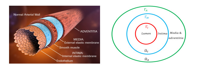
Atherosclerosis is a major cause of abdominal aortic aneurysm (AAA) and up to 80% of AAA patients have atherosclerosis. Therefore it is critical to understand the relationship and interactions between atherosclerosis and AAA to treat atherosclerotic aneurysm patients more effectively. In this paper, we develop a mathematical model to mimic the progression of atherosclerotic aneurysms by including both the multi-layer structured arterial wall and the pathophysiology of atherosclerotic aneurysms. The model is given by a system of partial differential equations with free boundaries. Our results reveal a 2D biomarker, the cholesterol ratio and DDR1 level, assessing the risk of atherosclerotic aneurysms. The efficacy of different treatment plans is also explored via our model and suggests that the dosage of anti-cholesterol drugs is significant to slow down the progression of atherosclerotic aneurysms while the additional anti-DDR1 injection can further reduce the risk.
Citation: Guoyi Ke, Chetan Hans, Gunjan Agarwal, Kristine Orion, Michael Go, Wenrui Hao. Mathematical model of atherosclerotic aneurysm[J]. Mathematical Biosciences and Engineering, 2021, 18(2): 1465-1484. doi: 10.3934/mbe.2021076
Atherosclerosis is a major cause of abdominal aortic aneurysm (AAA) and up to 80% of AAA patients have atherosclerosis. Therefore it is critical to understand the relationship and interactions between atherosclerosis and AAA to treat atherosclerotic aneurysm patients more effectively. In this paper, we develop a mathematical model to mimic the progression of atherosclerotic aneurysms by including both the multi-layer structured arterial wall and the pathophysiology of atherosclerotic aneurysms. The model is given by a system of partial differential equations with free boundaries. Our results reveal a 2D biomarker, the cholesterol ratio and DDR1 level, assessing the risk of atherosclerotic aneurysms. The efficacy of different treatment plans is also explored via our model and suggests that the dosage of anti-cholesterol drugs is significant to slow down the progression of atherosclerotic aneurysms while the additional anti-DDR1 injection can further reduce the risk.

| [1] |
J. Golledge, P. E. Norman, Atherosclerosis and abdominal aortic aneurysm: cause, response, or common risk factors?, Arterioscler. Thromb. Vasc. Biol., 30 (2010), 1075-1077. doi: 10.1161/ATVBAHA.110.206573

|
| [2] |
P. Libby, P. M. Ridker, G. K. Hansson, Progress and challenges in translating the biology of atherosclerosis, Nature, 473 (2011), 317-325. doi: 10.1038/nature10146
|
| [3] |
W. H. Pearce, V. P. Shively, Abdominal aortic aneurysm as a complex multifactorial disease: interactions of polymorphisms of inflammatory genes, features of autoimmunity, and current status of MMPs, Ann. N. Y. Acad. Sci., 1085 (2006), 117-132. doi: 10.1196/annals.1383.025
|
| [4] |
R. M. Sandford, M. J. Bown, N. J. London, R. D. Sayers, The genetic basis of abdominal aortic aneurysms: a review, Eur. J. Vasc. Endovasc. Surg., 33 (2007), 381-390. doi: 10.1016/j.ejvs.2006.10.025
|
| [5] |
S. Canic, Blood flow through compliant vessels after endovascular repair: wall deformations induced by the discontinuous wall properties, Comput. Vis. Sci., 4 (2002), 147-155. doi: 10.1007/s007910100066
|
| [6] | S. Canic, D. Mirkovic, A hyperbolic system of conservation laws in modeling endovascular treatment of abdominal aortic aneurysm, in Hyperbolic problems: theory, numerics, applications, Springer, (2001), 227-236. |
| [7] | S. Canic, K. Ravi-Chandar, Z. Krajcer, D. Mirkovic, S. Lapin, Mathematical model analysis of wallstent and aneurx: dynamic responses of bare-metal endoprosthesis compared with those of stent-graft, Tex. Heat I. J., 32 (2005), 502. |
| [8] | J. Chen, H. Huang, W. Hao, J. Xu, A machine learning method correlating pulse pressure wave data with pregnancy, Int. J. Numer. Meth. Bio., 36 (2020), e3272. |
| [9] |
P. Erhart, A. Hyhlik-Durr, P. Geisbusch, D. Kotelis, M. Muller-Eschner, T. C. Gasser, et al., Finite element analysis in asymptomatic, symptomatic, and ruptured abdominal aortic aneurysms: in search of new rupture risk predictors, Eur. J. Vasc. Endovasc. Surg., 49 (2015), 239-245. doi: 10.1016/j.ejvs.2014.11.010
|
| [10] | P. Fok, Growth of necrotic cores in atherosclerotic plaque, Math. Med. Biol., 29 (2011), 301-327. |
| [11] |
C. Poelma, P. N. Watton, Y. Ventikos, Transitional flow in aneurysms and the computation of haemodynamic parameters, J. R. Soc. Interface, 12 (2015), 20141394. doi: 10.1098/rsif.2014.1394
|
| [12] |
D. Roy, S. Lerouge, K. Inaekyan, C. Kauffmann, R. Mongrain, G. Soulez, Experimental validation of more realistic computer models for stent-graft repair of abdominal aortic aneurysms, including pre-load assessment, Int. J. Numer. Method. Biomed. Eng., 32 (2016), e02769. doi: 10.1002/cnm.2769
|
| [13] | E. Soudah, E. Y. Ng, T. H. Loong, M. Bordone, U. Pua, S. Narayanan, CFD modelling of abdominal aortic aneurysm on hemodynamic loads using a realistic geometry with CT, Comput. Math. Methods Med., 2013 (2013). |
| [14] |
J. Tambaa, M. Kosor, S. Canic, Mathematical modeling of vascular stents, SIAM J. Appl. Math., 70 (2010), 1922-1952. doi: 10.1137/080722618
|
| [15] |
F. Tian, L. Zhu, P. Fok, X. Lu, Simulation of a pulsatile non-newtonian flow past a stenosed 2d artery with atherosclerosis, Comput. Biol. Med., 43 (2013), 1098-1113. doi: 10.1016/j.compbiomed.2013.05.023
|
| [16] |
Q. Wang, A hydrodynamic theory for solutions of nonhomogeneous nematic liquid crystalline polymers of different configurations, J. Chem. Phys., 116 (2002), 9120-9136. doi: 10.1063/1.1452722
|
| [17] |
J. Wu, S. C. Shadden, Coupled Simulation of Hemodynamics and Vascular Growth and Remodeling in a Subject-Specific Geometr, Ann. Biomed. Eng., 43 (2015), 1543-1554. doi: 10.1007/s10439-015-1287-6
|
| [18] |
X. Yang, G. Forest, W. Mullins, Q. Wang, Dynamic defect morphology and hydrodynamics of sheared nematic polymers in two space dimensions, J. Rheol., 53 (2009), 589-615. doi: 10.1122/1.3089622
|
| [19] | Y. Yu, Fluid-structure interaction modeling in 3d cerebral arteries and aneurysms, in Biomedical Technology, Springer, (2018), 123-146. |
| [20] |
Y. Yu, P. Perdikaris, G. Karniadakis, Fractional modeling of viscoelasticity in 3d cerebral arteries and aneurysms, J. Comput. Phys., 323 (2016), 219-242. doi: 10.1016/j.jcp.2016.06.038
|
| [21] |
J. Zhao, X. Yang, J. Shen, Q. Wang, A decoupled energy stable scheme for a hydrodynamic phase-field model of mixtures of nematic liquid crystals and viscous fluids, J. Comput. Phys., 305 (2016), 539-556. doi: 10.1016/j.jcp.2015.09.044
|
| [22] |
M. Domanski, D. Lloyd-Jones, V. Fuster, S. Grundy, Can we dramatically reduce the incidence of coronary heart disease?, Nat. Rev. Cardiol., 8 (2011), 721-725. doi: 10.1038/nrcardio.2011.158
|
| [23] |
M. Dabagh, P. Jalali, J. M. Tarbell, Coupled Simulation of Hemodynamics and Vascular Growth and Remodeling in a Subject-Specific Geometr, Am. J. Physiol. Heart Circ. Physiol., 297 (2009), H983-H996. doi: 10.1152/ajpheart.00324.2009
|
| [24] |
M. Cilla, M. A. Martinez, E. Pena, Effect of Transmural Transport Properties on Atheroma Plaque
Formation and Development, Ann. Biomed. Eng., 43 (2015), 1516-1530. doi: 10.1007/s10439-015-1299-2
|
| [25] |
M. Cilla, E. Pena, M. A. Martinez, Mathematical modelling of atheroma plaque formation and development in coronary arteries, J. R. Soc. Interface, 11 (2014), 20130866. doi: 10.1098/rsif.2013.0866
|
| [26] |
K. Govindaraju, S. Kamangar, I. A. Badruddin, G. N. Viswanathan, A. Badarudin, N. J. Salman Ahmed, Effect of porous media of the stenosed artery wall to the coronary physiological diagnostic parameter: a computational fluid dynamic analysis, Atherosclerosis, 233 (2014), 630-635. doi: 10.1016/j.atherosclerosis.2014.01.043
|
| [27] |
A. Friedman, W. Hao, A Mathematical Model of Atherosclerosis with Reverse Cholesterol Transport and Associated Risk Factors, Bull. Math. Biol., 77 (2015), 758-781. doi: 10.1007/s11538-014-0010-3
|
| [28] |
W. Hao, A. Friedman, The LDL-HDL profile determines the risk of atherosclerosis: a mathematical model, PLoS One, 9 (2014), e90497. doi: 10.1371/journal.pone.0090497
|
| [29] |
D. A. Vorp, Biomechanics of abdominal aortic aneurysm, J. Biomech., 40 (2007), 1887-1902. doi: 10.1016/j.jbiomech.2006.09.003
|
| [30] |
D. A. Vorp, J. P. Vande Geest, Biomechanics of abdominal aortic aneurysm, Arterioscler. Thromb. Vasc. Biol., 25 (2005), 1558-1566. doi: 10.1161/01.ATV.0000174129.77391.55
|
| [31] |
V. Lobo, A. Patil, A. Phatak, N. Chandra, Free radicals, antioxidants and functional foods: Impact on human health, Pharmacogn. Rev., 4 (2010), 118-126. doi: 10.4103/0973-7847.70902
|
| [32] | K. T. Ji, L. Qian, J. L. Nan, Y. J. Xue, S. Q. Zhang, G. Q. Wang, et al., Ox-LDL induces dysfunction of endothelial progenitor cells via activation of NF-B, BioMed Res. Int., 2015 (2015). |
| [33] |
A. Rousselle, F. Qadri, L. Leukel, R. Yilmaz, J. F. Fontaine, G. Sihn, et al., CXCL5 limits
macrophage foam cell formation in atherosclerosis, J. Clin. Invest., 123 (2013), 1343-1347. doi: 10.1172/JCI66580
|
| [34] |
W. T. Gerthoffer, Mechanisms of vascular smooth muscle cell migration, Circ. Res., 100 (2007), 607-621. doi: 10.1161/01.RES.0000258492.96097.47
|
| [35] | G. Dimas, F. Iliadis, D. Grekas, Matrix metalloproteinases, atherosclerosis, proteinuria and kidney disease: Linkage-based approaches, Hippokratia, 17 (2013), 292-297. |
| [36] |
E. Galkina, K. Ley, Immune and inflammatory mechanisms of atherosclerosis, Annu. Rev. Immunol., 27 (2009), 165-197. doi: 10.1146/annurev.immunol.021908.132620
|
| [37] |
H. L. Fu, R. R. Valiathan, R. Arkwright, A. Sohail, C. Mihai, M. Kumarasiri, et al., Discoidin domain receptors: unique receptor tyrosine kinases in collagen-mediated signaling, J. Biol. Chem., 288 (2013), 7430-7437. doi: 10.1074/jbc.R112.444158
|
| [38] |
C. Franco, P. J. Ahmad, G. Hou, E. Wong, M. P. Bendeck, Increased cell and matrix accumulation during atherogenesis in mice with vessel wall-specific deletion of discoidin domain receptor 1, Circ. Res., 106 (2010), 1775-1783. doi: 10.1161/CIRCRESAHA.109.213637
|
| [39] |
W. L. Chan, N. Pejnovic, H. Hamilton, T. V. Liew, D. Popadic, A. Poggi, et al., Atherosclerotic
abdominal aortic aneurysm and the interaction between autologous human plaque-derived vascular
smooth muscle cells, type 1 NKT, and helper T cells, Circ. Res., 96 (2005), 675-683. doi: 10.1161/01.RES.0000160543.84254.f1
|
| [40] |
Q. Wang, J. Ren, S. Morgan, Z. Liu, C. Dou, B. Liu, Monocyte chemoattractant protein-1 (MCP-1)
regulates macrophage cytotoxicity in abdominal aortic aneurysm, PLoS One, 9 (2014), e92053. doi: 10.1371/journal.pone.0092053
|
| [41] |
W. Ma-Krupa, M. S. Jeon, S. Spoerl, T. F. Tedder, J. J. Goronzy, C. M. Weyand, Activation of arterial wall dendritic cells and breakdown of self-tolerance in giant cell arteritis, J. Exp. Med., 199 (2004), 173-183. doi: 10.1084/jem.20030850
|
| [42] | Q. Wang, C. Shu, J. Su, X. Li, A crosstalk triggered by hypoxia and maintained by MCP-1/miR- 98/IL-6/p38 regulatory loop between human aortic smooth muscle cells and macrophages leads to aortic smooth muscle cells apoptosis via Stat1 activation, Int. J. Clin. Exp. Pathol., 8 (2015), 2670-2679. |
| [43] | S. Becker, M. Warren, S. Haskill, Colony-stimulating factor-induced monocyte survival and differentiation into macrophages in serum-free cultures, J. Immun., 139 (1987), 3703-3709. |
| [44] |
C. S. Robbins, I. Hilgendorf, G. F. Weber, I. Theurl, Y. Iwamoto, J.-L. Figueiredo, et al., Local proliferation dominates lesional macrophage accumulation in atherosclerosis, Nat. Med., 19 (2013), 1166. doi: 10.1038/nm.3258
|
| [45] |
P. J. Gough, D. R. Greaves, H. Suzuki, T. Hakkinen, M. O. Hiltunen, M. Turunen, et al., Analysis of macrophage scavenger receptor (sr-a) expression in human aortic atherosclerotic lesions, Arterioscler. Thromb. Vasc. Biol., 19 (1999), 461-471. doi: 10.1161/01.ATV.19.3.461
|
| [46] |
C. Franco, K. Britto, E. Wong, G. Hou, S.-N. Zhu, M. Chen, et al., Discoidin domain receptor 1 on bone marrow-derived cells promotes macrophage accumulation during atherogenesis, Circ. Res., 105 (2009), 1141-1148. doi: 10.1161/CIRCRESAHA.109.207357
|
| [47] |
P. Wiesner, M. Tafelmeier, D. Chittka, S.-H. Choi, L. Zhang, Y. S. Byun, et al., Mcp-1 binds to oxidized ldl and is carried by lipoprotein (a) in human plasma, J. Lipid Res., 54 (2013), 1877-1883. doi: 10.1194/jlr.M036343
|
| [48] |
C. Franco, G. Hou, P. J. Ahmad, E. Y. Fu, L. Koh, W. F. Vogel, et al., Discoidin domain receptor 1 (ddr1) deletion decreases atherosclerosis by accelerating matrix accumulation and reducing inflammation in low-density lipoprotein receptor-deficient mice, Circ. Res., 102 (2008), 1202-1211. doi: 10.1161/CIRCRESAHA.107.170662
|
| [49] |
E. Raines, R. Ross, Smooth muscle cells and the pathogenesis of the lesions of atherosclerosis, Br. Heart J., 69 (1993), S30. doi: 10.1136/hrt.69.1_Suppl.S30
|
| [50] |
M. G. Watson, H. M. Byrne, C. Macaskill, M. R. Myerscough, A multiphase model of growth factor-regulated atherosclerotic cap formation, J. Math. Biol., 81 (2020), 725-767. doi: 10.1007/s00285-020-01526-6
|
| [51] |
R. Ross, Atherosclerosis-an inflammatory disease, N. Engl. J. Med., 340 (1999), 115-126. doi: 10.1056/NEJM199901143400207
|
| [52] |
D. Liu, L. Guan, Y. Zhao, Y. Liu, X. Sun, H. Li, et al., Association of triglycerides to high-density lipoprotein-cholesterol ratio with risk of incident hypertension}, Hypertens. Res., 43 (2020), 948-955. doi: 10.1038/s41440-020-0439-8
|
| [53] |
W. Masson, T. Epstein, M. Huerín, M. Lobo, G. Molinero, D. Siniawski, Association between
non-HDL-C/HDL-C ratio and carotid atherosclerosis in postmenopausal middle-aged women, Climacteric, 22 (2019), 518-522. doi: 10.1080/13697137.2019.1631787
|
| [54] |
W. Hao, S. Gong, S. Wu, J. Xu, M. R. Go, A. Friedman, et al., A mathematical model of aortic aneurysm formation, PLoS One, 12 (2017), e0170807. doi: 10.1371/journal.pone.0170807
|
| [55] | C. De Moura, C. Kubrusly, The courant-friedrichs-lewy (cfl) condition, AMC, 10 (2013), 12. |
| [56] |
T. C. Hodges, P. R. Detmer, D. L. Dawson, R. O. Bergelin, K. W. Beach, T. S. Hatsukami, et al., Ultrasound determination of total arterial wall thickness, J. Vasc. Surg., 19 (1994), 745-753. doi: 10.1016/S0741-5214(94)70051-6
|
| [57] |
C. Ciavarella, E. Gallitto, F. Ricci, M. Buzzi, A. Stella, G. Pasquinelli, The crosstalk between
vascular MSCs and inflammatory mediators determines the pro-calcific remodelling of human
atherosclerotic aneurysm, Stem Cell Res. Ther., 8 (2017), 99. doi: 10.1186/s13287-017-0554-x
|
| [58] |
A. R. Brady, S. G. Thompson, F. G. Fowkes, R. M. Greenhalgh, J. T. Powell, Abdominal aortic aneurysm expansion: risk factors and time intervals for surveillance, Circulation, 110 (2004), 16-21. doi: 10.1161/01.CIR.0000133279.07468.9F
|
| [59] |
R. W. Alexander, Hypertension and the pathogenesis of atherosclerosis: oxidative stress and the
mediation of arterial inflammatory response: a new perspective, Hypertension, 25 (1995), 155-161. doi: 10.1161/01.HYP.25.2.155
|
| [60] |
G. R. Gadowski, M. A. Ricci, E. D. Hendley, D. B. Pilcher, Hypertension accelerates the growth of experimental aortic aneurysms, J. Surg. Res., 54 (1993), 431-436. doi: 10.1006/jsre.1993.1068
|
| [61] | G. F. Mureddu, Arterial hypertension. Does the J curve exist? And then?, Monaldi Arch. Chest Dis., 88 (2018), 953. |
| [62] |
W. Hao, E. D. Crouser, A. Friedman, Mathematical model of sarcoidosis, PANS, 111 (2014), 16065-16070. doi: 10.1073/pnas.1417789111
|
| [63] |
W. Hao, H. M. Komar, P. A. Hart, D. L. Conwell, G. B. Lesinski, A. Friedman, Mathematical model of chronic pancreatitis, PNAS, 114 (2017), 5011-5016. doi: 10.1073/pnas.1620264114
|
| [64] |
T. Khamdaeng, J. Luo, J. Vappou, P. Terdtoon, E. E. Konofagou, Arterial stiffness identification of the human carotid artery using the stress-strain relationship in vivo, Ultrasonics, 52 (2012), 402-411. doi: 10.1016/j.ultras.2011.09.006
|
| [65] |
S. Laurent, Arterial wall hypertrophy and stiffness in essential hypertensive patients, Hypertension, 26 (1995), 355-362. doi: 10.1161/01.HYP.26.2.355
|
| [66] |
J. Xiong, S. M. Wang, W. Zhou, J. G. Wu, Measurement and analysis of ultimate mechanical properties, stress-strain curve fit, and elastic modulus formula of human abdominal aortic aneurysm and nonaneurysmal abdominal aorta, J. Vasc. Surg., 48 (2008), 189-195. doi: 10.1016/j.jvs.2007.12.053
|
| [67] |
Y. Momiyama, R. Ohmori, Z. A. Fayad, N. Tanaka, R. Kato, H. Taniguchi, et al., The LDLcholesterol to HDL-cholesterol ratio and the severity of coronary and aortic atherosclerosis, Atherosclerosis, 222 (2012), 577-580. doi: 10.1016/j.atherosclerosis.2012.03.023
|
| [68] | D. Moris, E. Mantonakis, E. Avgerinos, M. Makris, C. Bakoyiannis, E. Pikoulis, et al., Novel biomarkers of abdominal aortic aneurysm disease: identifying gaps and dispelling misperceptions, BioMed Res. Int., 2014 (2014). |
| [69] |
J. R. Tonniges, B. Albert, E. P. Calomeni, S. Roy, J. Lee, X. Mo, et al., Collagen Fibril Ultrastructure in Mice Lacking Discoidin Domain Receptor 1, Microsc. Microanal., 22 (2016), 599-611. doi: 10.1017/S1431927616000787
|
| [70] |
C. Franco, G. Hou, P. J. Ahmad, E. Y. Fu, L. Koh, W. F. Vogel, et al., Discoidin domain receptor
1 (ddr1) deletion decreases atherosclerosis by accelerating matrix accumulation and reducing inflammation in low-density lipoprotein receptor-deficient mice, Circ. Res., 102 (2008), 1202-1211. doi: 10.1161/CIRCRESAHA.107.170662
|
| [71] |
S. Xu, S. Bala, M. P. Bendeck, Discoidin domain receptor 1 deficiency in vascular smooth muscle
cells leads to mislocalisation of N-cadherin contacts, Biol. Open, 8 (2019), bio041913. doi: 10.1242/bio.041913
|
| [72] |
N. Ferri, N. O. Carragher, E. W. Raines, Role of discoidin domain receptors 1 and 2 in human
smooth muscle cell-mediated collagen remodeling: potential implications in atherosclerosis and
lymphangioleiomyomatosis, Am. J. Pathol., 164 (2004), 1575-1585. doi: 10.1016/S0002-9440(10)63716-9
|
| [73] |
G. Hou, W. Vogel, M. P. Bendeck, The discoidin domain receptor tyrosine kinase DDR1 in arterial
wound repair, J. Clin. Invest., 107 (2001), 727-735. doi: 10.1172/JCI10720
|
| [74] |
G. Hou, W. F. Vogel, M. P. Bendeck, Tyrosine kinase activity of discoidin domain receptor 1 is necessary for smooth muscle cell migration and matrix metalloproteinase expression, Circ. Res., 90 (2002), 1147-1149. doi: 10.1161/01.RES.0000022166.74073.F8
|
| [75] | T. Islam, Impact of statins on vascular smooth muscle cells and relevance to atherosclerosis, J. Physiol., (2020). |
| [76] |
H. Martynowicz, P. Gać, O. Kornafel-Flak, S. Filipów, Ł. Łaczmański, M. Sobieszczańska, et al., The relationship between the effectiveness of blood pressure control and telomerase reverse transcriptase concentration, adipose tissue hormone concentration and endothelium function in hypertensives, Heart Lung Circ., 29 (2020), e200-e209. doi: 10.1016/j.hlc.2019.12.012
|
| [77] | A. L. Høgh, J. Sandermann, J. S. Lindholt, Medical treatment of small abdominal aortic aneurysms, Ugeskr. Laeg., 170 (2008), 2003-2005. |
| [78] |
L. Castro-Sanchez, A. Soto-Guzman, M. Guaderrama-Diaz, P. Cortes-Reynosa, E. P. Salazar, Role
of DDR1 in the gelatinases secretion induced by native type IV collagen in MDA-MB-231 breast
cancer cells, Clin. Exp. Metastasis, 28 (2011), 463-477. doi: 10.1007/s10585-011-9385-9
|


Figures(8) / Tables(2)

Guoyi Ke, Chetan Hans, Gunjan Agarwal, Kristine Orion, Michael Go, Wenrui Hao. Mathematical model of atherosclerotic aneurysm[J]. Mathematical Biosciences and Engineering, 2021, 18(2): 1465-1484. doi: 10.3934/mbe.2021076


 DownLoad: