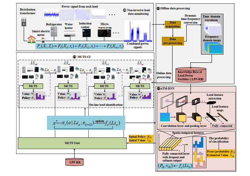
Cognitive green computing (CGC) is widely used in the Internet of Things (IoT) for the smart city. As the power system of the smart city, the smart grid has benefited from CGC, which can achieve the dynamic regulation of the electric energy and resource integration optimization. However, it is still challenging for improving the identification accuracy and the performance of the load model in the smart grid. In this paper, we present a novel algorithm framework based on reinforcement learning (RL) to improve the performance of non-invasive load monitoring and identification (NILMI). In this model, a knowledge base of load power facilities (LPF-KB) architecture is designed to facilitate the load data-shared collection and storage; utilizing deep convolutional neural networks (DNNs) structure based on the attentional mechanism to enhance the representations learning of load features; using RL-based Monte-Carlo tree search (MCTS) method to construct an optimal strategy network, and to realize the online combined load prediction without relying on the prior knowledge. We use the massive experiment on the real-world datasets of household appliances to evaluate the performance of our method. The experimental results show that our approach has remarkable performance in reducing the load online identification error rate. Our model is a generic model, and it can be widely used in practical load monitoring identification and the power prediction system.
Citation: Yanmei Jiang, Mingsheng Liu, Jianhua Li, Jingyi Zhang. Reinforced MCTS for non-intrusive online load identification based on cognitive green computing in smart grid[J]. Mathematical Biosciences and Engineering, 2022, 19(11): 11595-11627. doi: 10.3934/mbe.2022540
Cognitive green computing (CGC) is widely used in the Internet of Things (IoT) for the smart city. As the power system of the smart city, the smart grid has benefited from CGC, which can achieve the dynamic regulation of the electric energy and resource integration optimization. However, it is still challenging for improving the identification accuracy and the performance of the load model in the smart grid. In this paper, we present a novel algorithm framework based on reinforcement learning (RL) to improve the performance of non-invasive load monitoring and identification (NILMI). In this model, a knowledge base of load power facilities (LPF-KB) architecture is designed to facilitate the load data-shared collection and storage; utilizing deep convolutional neural networks (DNNs) structure based on the attentional mechanism to enhance the representations learning of load features; using RL-based Monte-Carlo tree search (MCTS) method to construct an optimal strategy network, and to realize the online combined load prediction without relying on the prior knowledge. We use the massive experiment on the real-world datasets of household appliances to evaluate the performance of our method. The experimental results show that our approach has remarkable performance in reducing the load online identification error rate. Our model is a generic model, and it can be widely used in practical load monitoring identification and the power prediction system.

| [1] |
D. P. M. Abellana, A systemic analysis of green computing adoption using genetically evolved fuzzy cognitive map: A Philippine scenario, Kybernetes, 50 (2020), 2668–2696. https://doi.org/10.1108/K-05-2020-0263 doi: 10.1108/K-05-2020-0263

|
| [2] |
W. M. Zheng, Q. W. Chai, J. hang, X. S. Xue, Ternary compound ontology matching for cognitive green computing, Math. Biosci. Eng., 18 (2021), 4860–4870. https://doi.org/10.3934/mbe.2021247 doi: 10.3934/mbe.2021247
|
| [3] |
X. Liu, Y. Li, X. Zhang, W. Lu, M. Xiong, Energy-efficient resource optimization in green cognitive internet of things, Mobile Networks Appl., 25 (2020), 107750–107770. https://doi.org/10.1007/s11036-020-01510-w doi: 10.1007/s11036-020-01510-w
|
| [4] |
Y. M. Jiang, M. S. Liu, H. Peng, M. Z. A. Bhuiyan, A reliable deep learning-based algorithm design for IoT load identification in smart grid, Ad Hoc Networks, 123 (2021), 102643–102673. https://doi.org/10.1016/j.adhoc.2021.102643 doi: 10.1016/j.adhoc.2021.102643
|
| [5] |
Y. Liu, L. Zhong, J. Qiu, J. Lu, W. Wang, Unsupervised domain adaptation for non-intrusive load monitoring via adversarial and joint adaptation network, IEEE Trans. Ind. Inf., 18 (2021), 266–277. https://doi.org/10.1109/TII.2021.3065934 doi: 10.1109/TII.2021.3065934
|
| [6] |
H. Peng, J. X. Li, S. Z. Wang, L. H. Wang, Q. R. Gong, R. Y. Yang, et al., Hierarchical taxonomy-aware and attentional graph capsule RCNNs for large-scale multi-label text classification, IEEE Trans. Knowl. Data Eng., 33 (2021), 2505–2519 https://doi.org/10.1109/TKDE.2019.2959991 doi: 10.1109/TKDE.2019.2959991
|
| [7] |
A. F. Moreno Jaramillo, D. M. Laverty, D. J. Morrow, J. Martinez del Rincon, A. M. Foley, Load modelling and non-intrusive load monitoring to integrate distributed energy resources in low and medium voltage networks, Renewable Energy, 179 (2021), 445–466. https://doi.org/10.1016/j.renene.2021.07.056 doi: 10.1016/j.renene.2021.07.056
|
| [8] |
R. V. A. Monteiro, J. C. R. de Santana, R. F. S. Teixeira, A. S. Bretas, R. Aguiar, C. E. P. Poma, Non-intrusive load monitoring using artificial intelligence classifiers: Performance analysis of machine learning techniques, Electr. Power Syst. Res., 198 (2021), 107347. https://doi.org/10.1016/j.epsr.2021.107347 doi: 10.1016/j.epsr.2021.107347
|
| [9] |
H. X. Wang, J. S. Zhang, C. B. Lu, C. Y. Wu, Privacy preserving in non-intrusive load monitoring: A differential privacy perspective, IEEE Trans. Smart Grid, 12 (2020), 2529–2543. https://doi.org/10.1109/TSG.2020.3038757 doi: 10.1109/TSG.2020.3038757
|
| [10] |
D. Hua, F. Q. Huang, L. J. Wang, W. T. Chen, Simultaneous disaggregation of multiple appliances based on non-intrusive load monitoring, Electr. Power Syst. Res., 193 (2021), 106887. https://doi.org/10.1016/j.epsr.2020.106887 doi: 10.1016/j.epsr.2020.106887
|
| [11] |
M. Dincecco, S. Squartini, M. J. Zhong, Transfer learning for non-intrusive load monitoring, IEEE Trans. Smart Grid, 11 (2020), 1419-1429. https://doi.org/10.1109/TSG.2019.2938068 doi: 10.1109/TSG.2019.2938068
|
| [12] |
G. A. Raiker, R. B. Subba, U. Loganathan, S. Agrawal, A. S. Thakur, J. P. Barton, et al., Energy disaggregation using energy demand model and IoT based control, IEEE Trans. Ind. Appl., 57 (2020), 1746–1754. https://doi.org/10.1109/TIA.2020.3047016 doi: 10.1109/TIA.2020.3047016
|
| [13] |
F. Ciancetta, G. Bucci, E. Fiorucci, S. Mari, A. Fioravanti, A new convolutional neural network-based system for NILM applications, IEEE Trans. Instrum. Meas., 70 (2021), 1501112. https://doi.org/10.1109/TIM.2020.3035193 doi: 10.1109/TIM.2020.3035193
|
| [14] |
A. Faustine, L. Pereira, C. Klemenjak, Adaptive weighted recurrence graphs for appliance recognition in non-intrusive load monitoring, IEEE Trans. Smart Grid, 12 (2020), 398–406. https://doi.org/10.1109/TSG.2020.3010621 doi: 10.1109/TSG.2020.3010621
|
| [15] |
Y. Himeur, A. Alsalemi, F. Bensaali, A. Amira, An intelligent nonintrusive load monitoring scheme based on 2D phase encoding of power signals, Int. J. Intell. Syst., 36 (2020), 72–93. https://doi.org/10.1002/int.22292 doi: 10.1002/int.22292
|
| [16] |
Y. Yang, J. Zhong, W. Li, T. A. Gulliver, S. Li, Semisupervised multilabel deep learning based nonintrusive load monitoring in smart grids, IEEE Trans. Ind. Inf., 16 (2020), 6892–6902. https://doi.org/10.1109/TII.2019.2955470 doi: 10.1109/TII.2019.2955470
|
| [17] |
M. Kaselimi, N. Doulamis, A. Voulodimos, E. Protopapadakis, A. Doulamis, Context aware energy disaggregation using adaptive bidirectional LSTM models, IEEE Trans. Smart Grid, 11 (2020), 3054–3067. https://doi.org/10.1109/TSG.2020.2974347 doi: 10.1109/TSG.2020.2974347
|
| [18] |
H. Chen, Y. H. Wang, C. H. Fan, A convolutional autoencoder-based approach with batch normalization for energy disaggregation, J. Supercomput., 11 (2021), 2961–2978. https://doi.org/10.1007/s11227-020-03375-y doi: 10.1007/s11227-020-03375-y
|
| [19] | P. Hao, J. Li, Y. He, Y. Liu, M. Bao, L. Wang, et al., Large-scale hierarchical text classification with recursively regularized deep graph-CNN, in Web Conference 2018: Proceedings of the 2018 World Wide Web Conference, Macao, Lyon, France, (2018), 1063–1072. https://doi.org/10.1145/3178876.3186005 |
| [20] | H. Peng, J. Li, Q. Gong, Y. Ning, S. Wang, L. He, Motif-matching based subgraph-level attentional convolutional network for graph classification, in Proceedings of the AAAI Conference on Artificial Intelligence, 34 (2021), 5387–5394. https://doi.org/10.1609/aaai.v34i04.5987 |
| [21] |
A. Moradzadeh, O. Sadeghian, K. Pourhossein, B. Mohammadiivatloo, A. Anvarimoghaddam, Improving residential load disaggregation for sustainable development of energy via principal component analysis, Sustainability, 12 (2020), 1–14. https://doi.org/10.3390/su12083158 doi: 10.3390/su12083158
|
| [22] | P. Hao, J. Li, Y. Song, Y. Liu, Incrementally learning the hierarchical softmax function for neural language models, in Thirty-First AAAI Conference on Artificial Intelligence, San Francisco, CA, 31 (2017), 3267–3273. https://doi.org/10.1609/aaai.v31i1.10994 |
| [23] |
A. U. Rehman, T. T. Lie, B. Vallès, S. R. Tito, Event-detection algorithms for low sampling nonintrusive load monitoring systems based on low complexity statistical features, IEEE Trans. Instrum. Meas., 69 (2019), 751–759. https://doi.org/10.1109/TIM.2019.2904351 doi: 10.1109/TIM.2019.2904351
|
| [24] |
M. S. Tsai, Y. H. Lin, Modern development of an adaptive non-intrusive appliance load monitoring system in electricity energy conservation, Appl. Energy, 96 (2012), 55–73. https://doi.org/10.1016/j.apenergy.2011.11.027 doi: 10.1016/j.apenergy.2011.11.027
|
| [25] |
Z. J. Zhou, Y. M. Xiang, H. Xu, Y. S. Wang, D. Shi, Z. W. Wang, Self-organizing probability neural network-based intelligent non-intrusive load monitoring with applications to low-cost residential measuring devices, Trans. Inst. Meas. Control, 96 (2020), 635–645. https://doi.org/10.1177/0142331220950865 doi: 10.1177/0142331220950865
|
| [26] |
C. Chen, P. Gao, J. Jiang, H. Wang, P. Li, S. Wan, A deep learning based non-intrusive household load identification for smart grid in China, Comput. Commun., 177 (2021), 175–184. https://doi.org/10.1016/j.comcom.2021.06.023 doi: 10.1016/j.comcom.2021.06.023
|
| [27] |
D. L. Su, Q. Shi, H. Xu, W. Wang, Nonintrusive load monitoring based on complementary features of spurious emissions, Electronics, 8 (2019), 1002. https://doi.org/10.3390/electronics8091002 doi: 10.3390/electronics8091002
|
| [28] |
F. Ciancetta, G. Bucci, E. Fiorucci, S. Mari, A. Fioravanti, A new convolutional neural network-based system for NILM applications, IEEE Trans. Instrum. Meas., 70 (2020), 1501112. https://doi.org/10.1109/TIM.2020.3035193 doi: 10.1109/TIM.2020.3035193
|
| [29] |
D. Ding, J. Li, K. Zhang, H. Wang, K. Wang, T. Cao, Non-intrusive load monitoring method with inception structured CNN, Appl. Intell., 30 (2021), 1–18. https://doi.org/10.1007/s10489-021-02690-y doi: 10.1007/s10489-021-02690-y
|
| [30] |
H. Peng, J. Li, Y. Song, R. Yang, R. Ranjan, P. S. Yu, et al., Streaming social event detection and evolution discovery in heterogeneous information networks, ACM Trans. Knowl. Discovery Data, 15 (2021), 1–33. https://doi.org/10.1145/3447585 doi: 10.1145/3447585
|
| [31] |
Z. Jia, L. Yang, Z. Zhang, H. Liu, F. Kong, Sequence to point learning based on bidirectional dilated residual network for non-intrusive load monitoring, Int. J. Electr. Power Energy Syst., 129 (2021), 106837. https://doi.org/10.1016/j.ijepes.2021.106837 doi: 10.1016/j.ijepes.2021.106837
|
| [32] |
H. Peng, R. Zhang, Y. Dou, R. Yang, J. Zhang, P. S. Yu, Reinforced neighborhood selection guided multi-relational graph neural networks, ACM Trans. Inf. Syst., 40 (2021), 1–46. https://doi.org/10.1145/3490181 doi: 10.1145/3490181
|
| [33] |
C. Dinesh, S. Makonin, I. V. Bajić, Residential power forecasting using load identification and graph spectral clustering, IEEE Trans. Circuits Syst. II Express Briefs, 66 (2019), 1900–1904. https://doi.org/10.1109/TCSII.2019.2891704 doi: 10.1109/TCSII.2019.2891704
|
| [34] | H. Peng, J. Li, Z. Wang, R. Yang, M. Liu, M. Zhang, et al., Lifelong property price prediction: A case study for the toronto real estate market, IEEE Trans. Knowl. Data Eng., 40 (2021). https://doi.org/10.1109/TKDE.2021.3112749 |
| [35] |
Z. Wu, C. Wang, H. Zhang, W. Peng, W. Liu, A time-efficient factorial hidden Semi-Markov model for non-intrusive load monitoring, Electr. Power Syst. Res., 199 (2021), 107372. https://doi.org/10.1016/j.epsr.2021.107372 doi: 10.1016/j.epsr.2021.107372
|
| [36] |
N. Henao, K. Agbossou, S. Kelouwani, Y. Dubé, M. Fournier, Approach in nonintrusive type I load monitoring using subtractive clustering, IEEE Trans. Smart Grid, 8 (2017), 812–821. https://doi.org/10.1109/TSG.2015.2462719 doi: 10.1109/TSG.2015.2462719
|
| [37] |
D. Yang, X. Gao, L. Kong, Y. Pang, B. Zhou, An event-driven convolutional neural architecture for non-intrusive load monitoring of residential appliance, IEEE Trans. Consum. Electron., 66 (2020), 173–182. https://doi.org/10.1109/TCE.2020.2977964 doi: 10.1109/TCE.2020.2977964
|
| [38] |
T. T. H. Le, S. Heo, H. Kim, Toward load identification based on the hilbert transform and sequence to sequence long short-term memory, IEEE Trans. Smart Grid, 12 (2021), 3252–3264. https://doi.org/10.1109/TSG.2021.3066570 doi: 10.1109/TSG.2021.3066570
|
| [39] |
H. Rafiq, X. Shi, H. Zhang, H. Li, M. K. Ochani, A. A. Shah, Generalizability improvement of deep learning based non-intrusive load monitoring system using data augmentation, IEEE Trans. Smart Grid, 99 (2021), 75–114. https://doi.org/10.1109/TSG.2021.3082622 doi: 10.1109/TSG.2021.3082622
|
| [40] |
S. Makonin, F. Popowich, I. V. Bajić, B. Gill, L. Bartram, Exploiting HMM sparsity to perform online real-time nonintrusive load monitoring, IEEE Trans. Smart Grid, 7 (2016), 2575–2585. https://doi.org/10.1109/TSG.2015.2494592 doi: 10.1109/TSG.2015.2494592
|
| [41] |
S. P. Cai, Z. M. Sun, J. Yan, D. H. Tang, Y. Chen, Z. Y. Zhou, Fisher information and online SVR-based dynamic modeling methodology for meteorological sensitive load forecasting in smart grids, IEEE Trans. Smart Grid, 104 (2021), 513–527. https://doi.org/10.1007/s00202-021-01308-3 doi: 10.1007/s00202-021-01308-3
|
| [42] |
V. Álvarez, S. Mazuelas, J. A. Lozano, Probabilistic load forecasting based on adaptive online learning, IEEE Trans. Smart Grid, 36 (2021), 3668–3680. https://doi.org/10.1109/TPWRS.2021.3050837 doi: 10.1109/TPWRS.2021.3050837
|
| [43] |
Y. Du, F. Li, Intelligent multi-microgrid energy management based on deep neural network and model-free reinforcement learning, IEEE Trans. Smart Grid, 11 (2019), 1066–1076. https://doi.org/10.1109/TSG.2019.2930299 doi: 10.1109/TSG.2019.2930299
|
| [44] |
C. Wang, S. Mei, H. Yu, S. Cheng, L. Du, P. Yang, Unintentional islanding transition control strategy for three-/single-phase multimicrogrids based on artificial emotional reinforcement learning, IEEE Syst. J., 15 (2021), 5464–5475. https://doi.org/10.1109/JSYST.2021.3074296 doi: 10.1109/JSYST.2021.3074296
|
| [45] |
H. Peng, H. Wang, B. Du, M. Bhuiyan, H. Ma, J. Liu, et al., Spatial temporal incidence dynamic graph neural networks for traffic flow forecasting, Inf. Sci., 521 (2020), 277–290. https://doi.org/10.1016/j.ins.2020.01.043 doi: 10.1016/j.ins.2020.01.043
|
| [46] | H. Peng, H. Li, Y. Song, V. W. Zheng, J. Li, Differentially private federated knowledge graphs embedding, IEEE Trans. Knowl. Data Eng., 40 (2021). https://doi.org/10.1145/3459637.3482252 |
| [47] |
Y. Li, R. Wang, Z. Yang, Optimal scheduling of isolated microgrids using automated reinforcement learning-based multi-period forecasting, IEEE Trans. Sustainable Energy, 13 (2022), 159–169. https://doi.org/10.1109/TSTE.2021.3105529 doi: 10.1109/TSTE.2021.3105529
|
| [48] |
D. Cao, W. Hu, X. Xu, Q. Wu, Q. Huang, Z. Chen, et al., Deep reinforcement learning based approach for optimal power flow of distribution networks embedded with renewable energy and storage devices, J. Mod. Power Syst. Clean Energy, 9 (2021), 1101–1110. https://doi.org/10.35833/MPCE.2020.000557 doi: 10.35833/MPCE.2020.000557
|
| [49] | J. Li, H. Peng, Y. Cao, Y. Dou, H. Zhang, P. S. Yu, et al., Higher-order attribute-enhancing heterogeneous graph neural networks, IEEE Trans. Knowl. Data Eng., 40 (2021). https://doi.org/10.48550/arXiv.2104.07892 |
| [50] |
L. Xi, L. Zhou, L. Liu, D. Duan, Y. Xu, L. Yang, et al., A deep reinforcement learning algorithm for the power order optimization allocation of AGC in interconnected power grids, CSEE J. Power Energy Syst., 6 (2020), 712–723. https://doi.org/10.17775/CSEEJPES.2019.01840 doi: 10.17775/CSEEJPES.2019.01840
|
| [51] |
D. Silver, J. Schrittwieser, K. Simonyan, I. Antonoglou, A. Huang, A. Guez, et al., Mastering the game of Go without human knowledge, Nature, 550 (2017), 354–359. https://doi.org/10.1038/nature24270 doi: 10.1038/nature24270
|
| [52] |
R. Yao, X. Lu, H. Zhou, J. Lai, A novel category-specific pricing strategy for demand response in microgrids, IEEE Trans. Sustainable Energy, 12 (2020), 182–195. https://doi.org/10.1109/TSTE.2021.3106329 doi: 10.1109/TSTE.2021.3106329
|
| [53] |
Z. Xiao, C. Fan, J. Yuan, X. Xu, W. Gang, Comparison between artificial neural network and random forest for effective disaggregation of building cooling load, Case Stud. Therm. Eng., 28 (2021), 101589. https://doi.org/10.1016/j.csite.2021.101589 doi: 10.1016/j.csite.2021.101589
|
| [54] |
R. Yao, H. Zhou, D. Zhou, H. Zhang, State characteristic clustering for nonintrusive load monitoring with stochastic bhaviours in smart grids, Complexity, 2021 (2021), 8839595. https://doi.org/10.1155/2021/8839595 doi: 10.1155/2021/8839595
|
| [55] | H. Peng, J. Li, Q. Gong, Y. Song, P. S. Yu, Fine-grained event categorization with heterogeneous graph convolutional networks, in Twenty-Eighth International Joint Conference on Artificial Intelligence IJCAI-19, (2019), 3238–3245. https://doi.org/10.48550/arXiv.1906.04580 |
| [56] |
Y. J. Zhang, L. Yu, Z. J. Fang, N. N. Xiong, L. J. Zhang, H. Y. Tian, An end-to-end deep learning model for robust smooth filtering identification, Future Gener. Comput. Syst., 127 (2021), 182–195. https://doi.org/10.1016/j.future.2021.09.004 doi: 10.1016/j.future.2021.09.004
|
| [57] |
Q. Liu, K. M. Kamoto, X. Liu, M. Sun, N. Linge, Low-complexity non-intrusive load monitoring using unsupervised learning and generalized appliance models, IEEE Trans. Consum. Electron., 65 (2019), 28–37. https://doi.org/10.1109/TCE.2019.2891160 doi: 10.1109/TCE.2019.2891160
|
| [58] |
H. Shuai, H. He, Online scheduling of a residential microgrid via Monte-Carlo tree search and a learned model, IEEE Trans. Smart Grid, 12 (2020), 1073–1087. https://doi.org/10.1109/TSG.2020.3035127 doi: 10.1109/TSG.2020.3035127
|
| [59] |
T. Shao, H. Zhang, K. Cheng, K. Zhang, L. Bie, The hierarchical task network planning method based on Monte Carlo tree search, Knowl.-Based Syst., 225 (2021), 107067. https://doi.org/10.1016/j.knosys.2021.107067 doi: 10.1016/j.knosys.2021.107067
|
| [60] |
R. Lu, S. H. Hong, M. Yu, Demand response for home energy management using reinforcement learning and artificial neural network, IEEE Trans. Smart Grid, 10 (2019), 6629–6639. https://doi.org/10.1109/TSG.2019.2909266 doi: 10.1109/TSG.2019.2909266
|
| [61] |
V. de Carvalho Neiva Pinheiro, A. L. Francato, W. B. Powell, Reinforcement learning for electricity dispatch in grids with high intermittent generation and energy storage systems: A case study for the Brazilian grid, Int. J. Energy Res., 44 (2020), 8635–8653. https://doi.org/10.1002/er.5551 doi: 10.1002/er.5551
|
| [62] |
H. Shuai, H. He, Online scheduling of a residential microgrid via Monte-Carlo tree search and a learned model, IEEE Trans. Smart Grid, 12 (2020), 1073–1087. https://doi.org/10.1109/TSG.2020.3035127 doi: 10.1109/TSG.2020.3035127
|
| [63] |
X. Liu, A. Fotouhi, Formula-E race strategy development using artificial neural networks and Monte Carlo tree search, Neural Comput. Appl., 32 (2020), 15191–15207. https://doi.org/10.1007/s00521-020-04871-1 doi: 10.1007/s00521-020-04871-1
|
| [64] | E. J. Powley, P. I. Cowling, D. Whitehouse, Memory bounded Monte Carlo tree search, in Thirteenth Artificial Intelligence and Interactive Digital Entertainment Conference, 13 (2017), 94–100. Available from: https://ojs.aaai.org/index.php/AIIDE/article/view/12932. |
| [65] |
R. Bonfigli, A. Felicetti, E. Principi, M. Fagiani, S. Squartini, F. Piazza, Denoising autoencoders for non-intrusive load monitoring: Improvements and comparative evaluation, Energy Build., 158 (2018), 1461–1474. https://doi.org/10.1016/j.enbuild.2017.11.054 doi: 10.1016/j.enbuild.2017.11.054
|
| [66] |
Y. Himeur, A. Alsalemi, F. Bensaali, A. Amira, Smart non-intrusive appliance identification using a novel local power histogramming descriptor with an improved k-nearest neighbors classifier, Sustainable Cities Soc., 67 (2021), 102764. https://doi.org/10.1016/j.scs.2021.102764 doi: 10.1016/j.scs.2021.102764
|
| [67] |
L. D. Nolasco, A. E. Lazzaretti, B. M. Mulinari, DeepDFML-NILM: A new CNN-based architecture for detection, feature extraction and multi-label classification in NILM signals, IEEE Sens. J., 22 (2022), 501–509. https://doi.org/10.1109/JSEN.2021.3127322 doi: 10.1109/JSEN.2021.3127322
|
| [68] | Z. Huang, X. Wei, Y. Kai, Bidirectional LSTM-CRF models for sequence tagging, Comput. Sci., 2015 (2015). https://doi.org/10.48550/arXiv.1508.01991 |


Figures(16) / Tables(3)

Yanmei Jiang, Mingsheng Liu, Jianhua Li, Jingyi Zhang. Reinforced MCTS for non-intrusive online load identification based on cognitive green computing in smart grid[J]. Mathematical Biosciences and Engineering, 2022, 19(11): 11595-11627. doi: 10.3934/mbe.2022540


 DownLoad: