This study aimed to assess the knowledge, attitudes, and practices of diabetic patients in Arar, Saudi Arabia, regarding diabetic retinopathy (DR) and identify their primary sources of information.
This cross-sectional descriptive survey was conducted in Arar, Saudi Arabia, with a sample size of 535 participants recruited via convenient sampling. A pre-designed questionnaire assessed the knowledge, attitudes, and practices toward DR. The survey evaluated the knowledge (12 questions), attitudes, practices (7 questions), and sources of information on DR. Data were analyzed using STATA/SE, and Chi-square tests were used to assess relationships between variables. Statistical significance was set at p < 0.05.
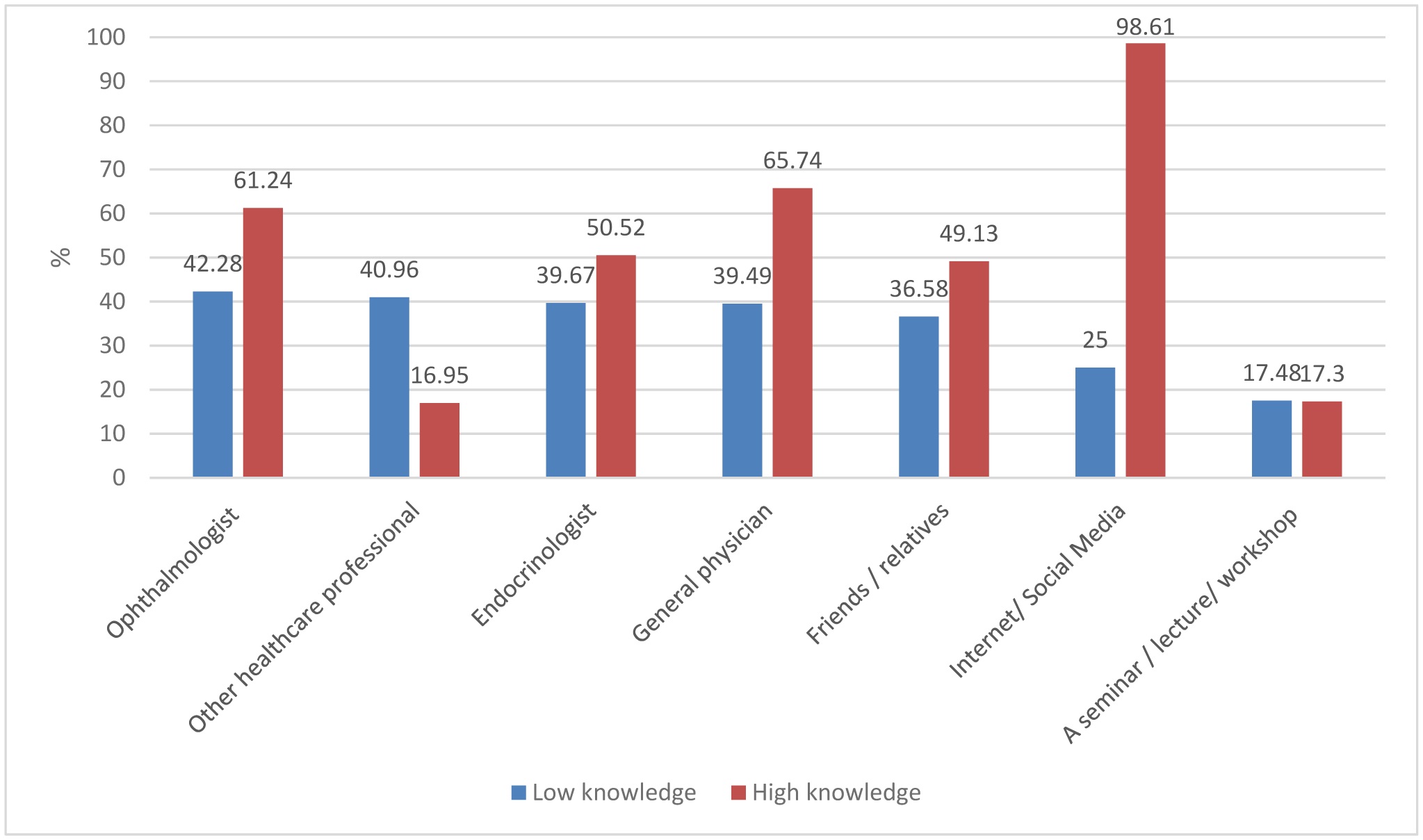
Of the 535 participants, 54% (289 participants) demonstrated a high knowledge, and 57% (305 participants) had positive attitudes and practices towards DR. Significant associations were found between the personal history of DR and both the knowledge and attitudes/practices (p < 0.001 each). The internet (71%) was the most common source of information, followed by general physicians (59%) and ophthalmologists (53%).
While most participants had a high knowledge and positive attitudes towards DR, there is room for improvement. A gap in understanding the impact of diabetes duration as a risk factor for DR was identified, thus highlighting the need for focused educational interventions. Enhancing health care professionals-patient communication and utilizing digital platforms can further raise awareness and promote preventive practices.
Citation: Mujeeb Ur Rehman Parrey, Hanaa El-Sayed Bayomy, Fawaz Salah M Alanazi, Asseel Farhan K Alanazi, Abdullah Hamoud M Alanazi, Abdulelah Raka A Alanazi. Diabetic retinopathy: knowledge, attitudes, and practices among diabetic patients[J]. AIMS Medical Science, 2025, 12(2): 210-222. doi: 10.3934/medsci.2025013
This study aimed to assess the knowledge, attitudes, and practices of diabetic patients in Arar, Saudi Arabia, regarding diabetic retinopathy (DR) and identify their primary sources of information.
This cross-sectional descriptive survey was conducted in Arar, Saudi Arabia, with a sample size of 535 participants recruited via convenient sampling. A pre-designed questionnaire assessed the knowledge, attitudes, and practices toward DR. The survey evaluated the knowledge (12 questions), attitudes, practices (7 questions), and sources of information on DR. Data were analyzed using STATA/SE, and Chi-square tests were used to assess relationships between variables. Statistical significance was set at p < 0.05.
Of the 535 participants, 54% (289 participants) demonstrated a high knowledge, and 57% (305 participants) had positive attitudes and practices towards DR. Significant associations were found between the personal history of DR and both the knowledge and attitudes/practices (p < 0.001 each). The internet (71%) was the most common source of information, followed by general physicians (59%) and ophthalmologists (53%).
While most participants had a high knowledge and positive attitudes towards DR, there is room for improvement. A gap in understanding the impact of diabetes duration as a risk factor for DR was identified, thus highlighting the need for focused educational interventions. Enhancing health care professionals-patient communication and utilizing digital platforms can further raise awareness and promote preventive practices.

| [1] |
Ansari P, Tabasumma N, Snigdha NN, et al. (2022) Diabetic retinopathy: an overview on mechanisms, pathophysiology and pharmacotherapy. Diabetology 3: 159-175. https://doi.org/10.3390/diabetology3010011 
|
| [2] |
Dal Canto E, Ceriello A, Rydén L, et al. (2019) Diabetes as a cardiovascular risk factor: an overview of global trends of macro and micro vascular complications. Eur J Prev Cardiol 26: 25-32. https://doi.org/10.1177/2047487319878371
|
| [3] |
Morya AK, Ramesh PV, Kaur K, et al. (2023) Diabetes more than retinopathy, it's effect on the anterior segment of eye. World J Clin Cases 11: 3736-3749. https://doi.org/10.12998/wjcc.v11.i16.3736
|
| [4] |
Li H, Liu X, Zhong H, et al. (2023) Research progress on the pathogenesis of diabetic retinopathy. BMC Ophthalmol 23: 372. https://doi.org/10.1186/s12886-023-03118-6
|
| [5] |
Son JW, Jang EH, Kim MK, et al. (2011) Diabetic retinopathy is associated with subclinical atherosclerosis in newly diagnosed type 2 diabetes mellitus. Diabetes Res Clin Pract 91: 253-259. https://doi.org/10.1016/j.diabres.2010.11.005
|
| [6] |
Li Z, Tong J, Liu C, et al. (2023) Analysis of independent risk factors for progression of different degrees of diabetic retinopathy as well as non-diabetic retinopathy among type 2 diabetic patients. Front Neurosci 17: 1143476. https://doi.org/10.3389/fnins.2023.1143476
|
| [7] | Sun Q, Jing Y, Zhang B, et al. (2021) The risk factors for diabetic retinopathy in a Chinese population: a cross-sectional study. J Diabetes Res 2021: 5340453. https://doi.org/10.1155/2021/5340453 |
| [8] |
Curtis TM, Gardiner TA, Stitt AW (2009) Microvascular lesions of diabetic retinopathy: clues towards understanding pathogenesis?. Eye 23: 1496-1508. https://doi.org/10.1038/eye.2009.108
|
| [9] | Bowling B (2015) Kanski's Clinical Ophthalmology: A Systemic Approach. 8th Eds., Edinburgh: Elsevier, 521. |
| [10] |
Kropp M, Golubnitschaja O, Mazurakova A, et al. (2023) Diabetic retinopathy as the leading cause of blindness and early predictor of cascading complications-risks and mitigation. EPMA J 14: 21-42. https://doi.org/10.1007/s13167-023-00314-8
|
| [11] |
Teo ZL, Tham YC, Yu M, et al. (2021) Global prevalence of diabetic retinopathy and projection of burden through 2045: systematic review and meta-analysis. Ophthalmology 128: 1580-1591. https://doi.org/10.1016/j.ophtha.2021.04.027
|
| [12] |
Parrey MU, Alswelmi FK (2017) Prevalence and causes of visual impairment among Saudi adults. Pak J Med Sci 33: 167-171. https://doi.org/10.12669/pjms.331.11871
|
| [13] |
Jarrar M, Abusalah MAH, Albaker W, et al. (2023) Prevalence of type 2 diabetes mellitus in the general population of saudi arabia, 2000–2020: a systematic review and meta-analysis of observational studies. Saudi J Med Med Sci 11: 1-10. https://doi.org/10.4103/sjmms.sjmms_394_22
|
| [14] |
Chung YC, Xu T, Tung TH, et al. (2022) Early screening for diabetic retinopathy in newly diagnosed type 2 diabetes and its effectiveness in terms of morbidity and clinical treatment: a nationwide population-based cohort. Front Public Health 10: 771862. https://doi.org/10.3389/fpubh.2022.771862
|
| [15] | Upadhyay T, Prasad R, Mathurkar S (2024) A narrative review of the advances in screening methods for diabetic retinopathy: enhancing early detection and vision preservation. Cureus 16: e53586. https://doi.org/10.7759/cureus.53586 |
| [16] |
AlHargan MH, AlBaker KM, AlFadhel AA, et al. (2019) Awareness, knowledge, and practices related to diabetic retinopathy among diabetic patients in primary healthcare centers at Riyadh, Saudi Arabia. J Family Med Prim Care 8: 373-377. https://doi.org/10.4103/jfmpc.jfmpc_422_18
|
| [17] |
Alzahrani SH, Bakarman MA, Alqahtani SM, et al. (2018) Awareness of diabetic retinopathy among people with diabetes in Jeddah, Saudi Arabia. Ther Adv Endocrinol Metab 9: 103-112. https://doi.org/10.1177/2042018818758621
|
| [18] | Alqahtani TF, Alqarehi R, Mulla OM, et al. (2023) Knowledge, attitude, and practice regarding diabetic retinopathy screening and eye management among diabetics in Saudi Arabia. Cureus 15: e46190. https://doi.org/10.7759/cureus.46190 |
| [19] | Al-Eryani SA, Al-Shamahi EY, AlShamahi EM, et al. (2023) Knowledge and awareness of diabetic retinopathy among diabetic patients in Sana'a City, Yemen. Ann Clin Case Rep 8: 2441. |
| [20] |
Hamzeh A, Almhanni G, Aljaber Y, et al. (2019) Awareness of diabetes and diabetic retinopathy among a group of diabetic patients in main public hospitals in Damascus, Syria during the Syrian crisis. BMC Health Serv Res 19: 549. https://doi.org/10.1186/s12913-019-4375-8
|
| [21] | Abdu M, Allinjawi K, Almabadi HM (2022) An assessment on the awareness of diabetic retinopathy among participants attending the diabetes awareness camp in Saudi Arabia. Cureus 14: e31031. https://doi.org/10.7759/cureus.31031 |
| [22] |
Qi JY, Zhai G, Wang Y, et al. (2022) Assessment of knowledge, attitude, and practice regarding diabetic retinopathy in an urban population in northeast China. Front Public Health 10: 808988. https://doi.org/10.3389/fpubh.2022.808988
|
Figures(1) / Tables(6)

Mujeeb Ur Rehman Parrey, Hanaa El-Sayed Bayomy, Fawaz Salah M Alanazi, Asseel Farhan K Alanazi, Abdullah Hamoud M Alanazi, Abdulelah Raka A Alanazi. Diabetic retinopathy: knowledge, attitudes, and practices among diabetic patients[J]. AIMS Medical Science, 2025, 12(2): 210-222. doi: 10.3934/medsci.2025013


 DownLoad: