At the end of 2022, a total of 20,003 diagnoses of human immunodeficiency virus (HIV) infection and 8,983 cases of acquired immunodeficiency syndrome (AIDS) among Japanese nationals, and 3,860 HIV diagnoses and 1,575 AIDS cases among foreign residents, had been notified to the government in Japan. This study updates the estimate of HIV incidence, including during the COVID-19 pandemic. It aimed to reconstruct the incidence of HIV and understand how the disruption caused by COVID-19 affected the epidemiology of HIV. Using a median incubation period of 10.0 years, the number of undiagnosed HIV infections was estimated to be 3,209 (95% confidence interval (CI): 2,642, 3,710) at the end of 2022. This figure has declined steadily over the past 10 years. Assuming that the median incubation period was 10.0 years, the proportion of diagnosed HIV infections, including surviving AIDS cases, was 89.3% (95% CI: 87.8%, 91.0%). When AIDS cases were excluded, the proportion was 86.2% (95% CI: 84.3%, 88.3%). During the COVID-19 pandemic, the estimated annual diagnosis rate was slightly lower than during earlier time intervals, at around 16.5% (95% CI: 14.9%, 18.1%). Japan may already have achieved diagnostic coverage of 90%, given its 9% increment in the diagnosed proportion during the past 5 years. The incidence of HIV infection continued to decrease even during the COVID-19 pandemic from 2020 to 2022, and the annual rate of diagnosis decreased slightly to 16.5%. Monitoring the recovery of diagnosis along with the effective reproduction number is vital in the future.
Citation: Hiroshi Nishiura, Seiko Fujiwara, Akifumi Imamura, Takuma Shirasaka. HIV incidence before and during the COVID-19 pandemic in Japan[J]. Mathematical Biosciences and Engineering, 2024, 21(4): 4874-4885. doi: 10.3934/mbe.2024215
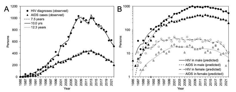
At the end of 2022, a total of 20,003 diagnoses of human immunodeficiency virus (HIV) infection and 8,983 cases of acquired immunodeficiency syndrome (AIDS) among Japanese nationals, and 3,860 HIV diagnoses and 1,575 AIDS cases among foreign residents, had been notified to the government in Japan. This study updates the estimate of HIV incidence, including during the COVID-19 pandemic. It aimed to reconstruct the incidence of HIV and understand how the disruption caused by COVID-19 affected the epidemiology of HIV. Using a median incubation period of 10.0 years, the number of undiagnosed HIV infections was estimated to be 3,209 (95% confidence interval (CI): 2,642, 3,710) at the end of 2022. This figure has declined steadily over the past 10 years. Assuming that the median incubation period was 10.0 years, the proportion of diagnosed HIV infections, including surviving AIDS cases, was 89.3% (95% CI: 87.8%, 91.0%). When AIDS cases were excluded, the proportion was 86.2% (95% CI: 84.3%, 88.3%). During the COVID-19 pandemic, the estimated annual diagnosis rate was slightly lower than during earlier time intervals, at around 16.5% (95% CI: 14.9%, 18.1%). Japan may already have achieved diagnostic coverage of 90%, given its 9% increment in the diagnosed proportion during the past 5 years. The incidence of HIV infection continued to decrease even during the COVID-19 pandemic from 2020 to 2022, and the annual rate of diagnosis decreased slightly to 16.5%. Monitoring the recovery of diagnosis along with the effective reproduction number is vital in the future.

| [1] | The Committee of AIDS Trends, Ministry of Health, Labour and Welfare. HIV/AIDS in Japan. Tokyo, Ministry of Health, Labour and Welfare. https://api-net.jfap.or.jp/status/japan/nenpo.html |
| [2] |
R. M. Granich, C. F. Gilks, C. Dye, K. M. De Cock, B. G. Williams, Universal voluntary HIV testing with immediate antiretroviral therapy as a strategy for elimination of HIV transmission: A mathematical model, Lancet (London, England), 373 (2009), 48–57. https://doi.org/10.1016/S0140-6736(08)61697-9 doi: 10.1016/S0140-6736(08)61697-9

|
| [3] |
R. Granich, B. Williams, J. Montaner, J. M. Zuniga, 90-90-90 and ending AIDS: Necessary and feasible. Lancet (London, England), 390 (2017), 341–343. https://doi.org/10.1016/S0140-6736(17)31872-X doi: 10.1016/S0140-6736(17)31872-X
|
| [4] |
C. Okoli, N. Van de Velde, B. Richman, B. Allan, E. Castellanos, B. Young, et al., Undetectable equals untransmittable (U = U): Awareness and associations with health outcomes among people living with HIV in 25 countries, Sexual. Transmit. Infect., 97 (2021), 18–26. https://doi.org/10.1136/sextrans-2020-054551 doi: 10.1136/sextrans-2020-054551
|
| [5] | G. Nair, C. Celum, D. Szydlo, E. R. Brown, et al., REACH Protocol Team, Adherence, safety, and choice of the monthly dapivirine vaginal ring or oral emtricitabine plus tenofovir disoproxil fumarate for HIV pre-exposure prophylaxis among African adolescent girls and young women: A randomised, open-label, crossover trial, Lancet. HIV, (2023), S2352-3018(23)00227-8. Advance online publication. https://doi.org/10.1016/S2352-3018(23)00227-8 |
| [6] | UNAIDS, An ambitious treatment target to help end the AIDS epidemic. https://www.unaids.org/sites/default/files/media_asset/90-90-90_en.pdf |
| [7] |
A. Iwamoto, R. Taira, Y. Yokomaku, T. Koibuchi, M. Rahman, Y. Izumi, et al., The HIV care cascade: Japanese perspectives, PloS One, 12 (2017), e0174360. https://doi.org/10.1371/journal.pone.0174360 doi: 10.1371/journal.pone.0174360
|
| [8] |
H. Nishiura, Estimating the incidence and diagnosed proportion of HIV infections in Japan: A statistical modeling study, PeerJ, 7 (2019), e6275. https://doi.org/10.7717/peerj.6275 doi: 10.7717/peerj.6275
|
| [9] |
K. Ejima, Y. Koizumi, N. Yamamoto, M. Rosenberg, C. Ludema, A. I. Bento, et al., HIV testing by public health centers and municipalities and new HIV cases during the COVID-19 pandemic in Japan, J. Acquir. Immune Deficiency Syndrom., 87 (2021), e182–e187. https://doi.org/10.1097/QAI.0000000000002660 doi: 10.1097/QAI.0000000000002660
|
| [10] |
R. Brookmeyer, M. H. Gail, Minimum size of the acquired immunodeficiency syndrome (AIDS) epidemic in the United States, Lancet (London, England), 2 (1986), 1320–1322. https://doi.org/10.1016/s0140-6736(86)91444-3 doi: 10.1016/s0140-6736(86)91444-3
|
| [11] |
R. Brookmeyer, J. J. Goedert, Censoring in an epidemic with an application to hemophilia-associated AIDS, Biometrics, 45 (1989), 325–335. https://doi.org/10.2307/2532057 doi: 10.2307/2532057
|
| [12] |
J. L. Boldsen, J. L. Jensen, J. Sogaard, M. Sorensen, On the incubation time distribution and the Danish AIDS data, J. Royal Statist. Soc. Series A (Stat. Soc.), 151 (1988), 42–43. https://doi.org/10.2307/2982183 doi: 10.2307/2982183
|
| [13] |
A. Muñoz, J. Xu, Models for the incubation of AIDS and variations according to age and period, Stat. Med., 15 (1966), 2459–2473. https://doi.org/10.1002/(sici)1097-0258(19961130)15:22<2459::aid-sim464>3.0.co;2-q doi: 10.1002/(sici)1097-0258(19961130)15:22<2459::aid-sim464>3.0.co;2-q
|
| [14] | UNAIDS. Global AIDS strategy 2021-2026. End inequalities. End AIDS. https://www.unaids.org/sites/default/files/media_asset/global-AIDS-strategy-2021-2026-summary_en.pdf |
| [15] |
E. Lee, J. Kim, J. Y. Lee, J. H. Bang, Estimation of the Number of HIV Infections and Time to Diagnosis in the Korea, J. Korean Med. Sci., 35 (2020), e41. https://doi.org/10.3346/jkms.2020.35.e41 doi: 10.3346/jkms.2020.35.e41
|
| [16] |
P. G. Patel, P. Keen, H. McManus, T. Duck, D. Callander, C. Selvey, et al., NSW HIV Prevention Partnership Project, Increased targeted HIV testing and reduced undiagnosed HIV infections among gay and bisexual men, HIV Med., 22 (2021), 605–616. https://doi.org/10.1111/hiv.13102 doi: 10.1111/hiv.13102
|
| [17] |
R. T. Gray, D. P. Wilson, R. J. Guy, M. Stoové, M. E. Hellard, G. P. Prestage, et al., Undiagnosed HIV infections among gay and bisexual men increasingly contribute to new infections in Australia, J. Int. AIDS Soc., 21 (2018), e25104. https://doi.org/10.1002/jia2.25104 doi: 10.1002/jia2.25104
|
| [18] | J. King, H. McManus, A. Kwon, R. Gray, S. McGregor, HIV, viral hepatitis and sexually transmissible infections in Australia: Annual surveillance report 2022, The Kirby Institute, UNSW Sydney, Sydney, Australia. http://doi.org/10.26190/sx44-5366 |
| [19] | AIDS Prevention Information Network. (n.d.). Annual Report on the Status of Deaf in Japan. Retrieved November 13, 2023, from https://api-net.jfap.or.jp/status/japan/nenpo.html |
| [20] | I. Itoda, T. Sano, M. Kondo, M. Imai, Implementing effective HIV testing at private clinics and improvement of the quality, Annual Research Report of the Health and Labour Research Grant, Ministry of Health, Labour and Welfare: Tokyo, 2022 (written in Japanese) |


Figures(4)

Hiroshi Nishiura, Seiko Fujiwara, Akifumi Imamura, Takuma Shirasaka. HIV incidence before and during the COVID-19 pandemic in Japan[J]. Mathematical Biosciences and Engineering, 2024, 21(4): 4874-4885. doi: 10.3934/mbe.2024215


 DownLoad: