Global dynamics of IAV/SARS-CoV-2 coinfection model with eclipse phase and antibody immunity

A. M. Elaiw; Raghad S. Alsulami; A. D. Hobiny; A. M. Elaiw; Raghad S. Alsulami; A. D. Hobiny

doi:10.3934/mbe.2023182

Mathematical Biosciences and Engineering

2023, Volume 20, Issue 2: 3873-3917. doi: 10.3934/mbe.2023182

Previous Article Next Article

Research article

Global dynamics of IAV/SARS-CoV-2 coinfection model with eclipse phase and antibody immunity

Department of Mathematics, Faculty of Science, King Abdulaziz University, P. O. Box 80203, Jeddah 21589, Saudi Arabia

Academic Editor: Yang Kuang

Received: 08 October 2022 Revised: 12 November 2022 Accepted: 25 November 2022 Published: 13 December 2022

Coronavirus disease 2019 (COVID-19) and influenza are two respiratory infectious diseases of high importance widely studied around the world. COVID-19 is caused by the severe acute respiratory syndrome coronavirus 2 (SARS-CoV-2), while influenza is caused by one of the influenza viruses, A, B, C, and D. Influenza A virus (IAV) can infect a wide range of species. Studies have reported several cases of respiratory virus coinfection in hospitalized patients. IAV mimics the SARS-CoV-2 with respect to the seasonal occurrence, transmission routes, clinical manifestations and related immune responses. The present paper aimed to develop and investigate a mathematical model to study the within-host dynamics of IAV/SARS-CoV-2 coinfection with the eclipse (or latent) phase. The eclipse phase is the period of time that elapses between the viral entry into the target cell and the release of virions produced by that newly infected cell. The role of the immune system in controlling and clearing the coinfection is modeled. The model simulates the interaction between nine compartments, uninfected epithelial cells, latent/active SARS-CoV-2-infected cells, latent/active IAV-infected cells, free SARS-CoV-2 particles, free IAV particles, SARS-CoV-2-specific antibodies and IAV-specific antibodies. The regrowth and death of the uninfected epithelial cells are considered. We study the basic qualitative properties of the model, calculate all equilibria, and prove the global stability of all equilibria. The global stability of equilibria is established using the Lyapunov method. The theoretical findings are demonstrated via numerical simulations. The importance of considering the antibody immunity in the coinfection dynamics model is discussed. It is found that without modeling the antibody immunity, the case of IAV and SARS-CoV-2 coexistence will not occur. Further, we discuss the effect of IAV infection on the dynamics of SARS-CoV-2 single infection and vice versa.
- COVID-19,
- SARS-CoV-2,
- influenza a virus,
- coinfection,
- global stability,
- Lyapunov function
Citation: A. M. Elaiw, Raghad S. Alsulami, A. D. Hobiny. Global dynamics of IAV/SARS-CoV-2 coinfection model with eclipse phase and antibody immunity[J]. Mathematical Biosciences and Engineering, 2023, 20(2): 3873-3917. doi: 10.3934/mbe.2023182

Related Papers:

Abstract

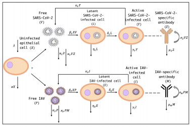
Coronavirus disease 2019 (COVID-19) and influenza are two respiratory infectious diseases of high importance widely studied around the world. COVID-19 is caused by the severe acute respiratory syndrome coronavirus 2 (SARS-CoV-2), while influenza is caused by one of the influenza viruses, A, B, C, and D. Influenza A virus (IAV) can infect a wide range of species. Studies have reported several cases of respiratory virus coinfection in hospitalized patients. IAV mimics the SARS-CoV-2 with respect to the seasonal occurrence, transmission routes, clinical manifestations and related immune responses. The present paper aimed to develop and investigate a mathematical model to study the within-host dynamics of IAV/SARS-CoV-2 coinfection with the eclipse (or latent) phase. The eclipse phase is the period of time that elapses between the viral entry into the target cell and the release of virions produced by that newly infected cell. The role of the immune system in controlling and clearing the coinfection is modeled. The model simulates the interaction between nine compartments, uninfected epithelial cells, latent/active SARS-CoV-2-infected cells, latent/active IAV-infected cells, free SARS-CoV-2 particles, free IAV particles, SARS-CoV-2-specific antibodies and IAV-specific antibodies. The regrowth and death of the uninfected epithelial cells are considered. We study the basic qualitative properties of the model, calculate all equilibria, and prove the global stability of all equilibria. The global stability of equilibria is established using the Lyapunov method. The theoretical findings are demonstrated via numerical simulations. The importance of considering the antibody immunity in the coinfection dynamics model is discussed. It is found that without modeling the antibody immunity, the case of IAV and SARS-CoV-2 coexistence will not occur. Further, we discuss the effect of IAV infection on the dynamics of SARS-CoV-2 single infection and vice versa.

References

[1]	World Health Organization (WHO), Coronavirus disease (COVID-19), weekly epidemiological update (2 October 2022), 2022. Available from: https://www.who.int/publications/m/item/weekly-epidemiological-update-on-covid-19—5-october-2022.
[2]	A. D. Iuliano, K. M. Roguski, H. H. Chang, D. J. Muscatello, R. Palekar, S. Tempia, et al., Estimates of global seasonal influenza-associated respiratory mortality: A modelling study, Lancet, 391 (2018), 1285–1300. https://doi.org/10.1016/S0140-6736(17)33293-2 doi: 10.1016/S0140-6736(17)33293-2
[3]	B. Hancioglu, D. Swigon, G. Clermont, A dynamical model of human immune response to influenza A virus infection, J. Theor. Biol., 246 (2007), 70–86. https://doi.org/10.1016/j.jtbi.2006.12.015 doi: 10.1016/j.jtbi.2006.12.015
[4]	Z. Varga, A. J. Flammer, P. Steiger, M. Haberecker, R. Andermatt, A. S. Zinkernagel, et al., Endothelial cell infection and endotheliitis in COVID-19, Lancet, 395 (2020), 1417–1418. https://doi.org/10.1016/S0140-6736(20)30937-5 doi: 10.1016/S0140-6736(20)30937-5
[5]	R. Ozaras, Influenza and COVID-19 coinfection: Report of six cases and review of the literature, J. Med. Virol, 92 (2020), 2657–2665. https://doi.org/10.1002/jmv.26125 doi: 10.1002/jmv.26125
[6]	World Health Organization (WHO), Influenza Update No. 428, (19 September 2022), 2022. Available from: https://www.who.int/publications/m/item/influenza-update-n-428.
[7]	World Health Organization (WHO), Coronavirus disease (COVID-19), Vaccine tracker, 2022. Available from: https://covid19.trackvaccines.org/agency/who/.
[8]	R. F. Nuwarda, A. A. Alharbi, V. Kayser, An overview of influenza viruses and vaccines, Vaccines, 9 (2021), 1032. https://doi.org/10.3390/vaccines9091032 doi: 10.3390/vaccines9091032
[9]	X. Zhu, Y. Gea, T. Wua, K. Zhaoa, Y. Chena, B. Wu, et al., Co-infection with respiratory pathogens among COVID-2019 cases, Virus Research, 285 (2020), 198005. https://doi.org/10.1016/j.virusres.2020.198005 doi: 10.1016/j.virusres.2020.198005
[10]	P. S. Aghbash, N. Eslami, M. Shirvaliloo, H. B. Baghi, Viral coinfections in COVID-19, J. Med. Virol., 93 (2021), 5310–5322. https://doi.org/10.1002/jmv.27102 doi: 10.1002/jmv.27102
[11]	Q. Ding, P. Lu, Y. Fan, Y. Xia, M. Liu, The clinical characteristics of pneumonia patients coinfected with 2019 novel coronavirus and influenza virus in Wuhan, China, J. Med. Virol., 92 (2020), 1549–1555. https://doi.org/10.1002/jmv.25781 doi: 10.1002/jmv.25781
[12]	G. Wang, M. Xie, J. Ma, J. Guan, Y. Song, Y. Wen, et al., Is co-infection with influenza virus a protective factor of COVID-19?, 2020.
[13]	M. Wang, Q. Wu, W. Xu, B. Qiao, J. Wang, H. Zheng, et al., Clinical diagnosis of 8274 samples with 2019-novel coronavirus in Wuhan, MedRxiv, (2020). https://doi.org/10.1101/2020.02.12.20022327
[14]	L. Lansbury, B. Lim, V. Baskaran, W. S. Lim, Co-infections in people with COVID-19: A systematic review and meta-analysis, J. Infect., 81 (2020), 266–275. https://doi.org/10.1016/j.jinf.2020.05.046 doi: 10.1016/j.jinf.2020.05.046
[15]	T. L. Dao, P. Colson, M. Million, P. Gautret, Co-infection of SARS-CoV-2 and influenza viruses: A systematic review and meta-analysis, J. Clin. Virol., 1 (2021), 100036. https://doi.org/10.1016/j.jcvp.2021.100036 doi: 10.1016/j.jcvp.2021.100036
[16]	H. Ghaznavi, M. Shirvaliloo, S. Sargazi, Z. Mohammadghasemipour, Z. Shams, Z. Hesari, et al., SARS-CoV-2 and influenza viruses: Strategies to cope with coinfection and bioinformatics perspective, CBI, 46 (2022), 1009–1020. https://doi.org/10.1002/cbin.11800 doi: 10.1002/cbin.11800
[17]	H. Khorramdelazada, M. H. Kazemib, A. Najafib, M. Keykhaeee, R. Z. Emameh, R. Falak, Immunopathological similarities between COVID-19 and influenza: Investigating the consequences of co-infection, Microb. Pathog., 152 (2021), 104554. https://doi.org/10.1016/j.micpath.2020.104554 doi: 10.1016/j.micpath.2020.104554
[18]	X. Xiang, Z. Wang, L. Ye, X. He, X. Wei, Y. Ma, et al., Co-infection of SARS-COV-2 and influenza A virus: A case series and fast review, Curr. Med. Sci.41 (2021), 51–57. https://doi.org/10.1007/s11596-021-2317-2
[19]	H. Yue, M. Zhang, L. Xing, K. Wang, X. Rao, H. Liu, et al., The epidemiology and clinical characteristics of co-infection of SARS-CoV-2 and influenza viruses in patients during COVID-19 outbreak, J. Med. Virol., 92 (2020), 2870–2873. https://doi.org/10.1002/jmv.26163 doi: 10.1002/jmv.26163
[20]	A. J. Zhang, A. C. Lee, J. F. Chan, F. Liu, C. Li, Y. Chen, H. Chu, et al., Coinfection by severe acute respiratory syndrome coronavirus 2 and influenza A (H1N1) pdm09 virus enhances the severity of pneumonia in golden Syrian hamsters, Clin. Infect. Dis., 72 (2021), e978–e992. https://doi.org/10.1093/cid/ciaa1747 doi: 10.1093/cid/ciaa1747
[21]	M. D. Nowak, E. M. Sordillo, M. R. Gitman, A. E. P. Mondolfi, Coinfection in SARS-CoV-2 infected patients: Where are influenza virus and rhinovirus/enterovirus?, J. Med. Virol., 92 (2020), 1699. https://doi.org/10.1002/jmv.25953 doi: 10.1002/jmv.25953
[22]	P. J. Halfmann, N. Nakajima, Y. Sato, K. Takahashi, M. Accola, S. Chiba, et al., SARS-CoV-2 interference of influenza virus replication in Syrian hamsters, JID, 225 (2022), 282–286. https://doi.org/10.1093/infdis/jiab587 doi: 10.1093/infdis/jiab587
[23]	K. Oishi, S. Horiuchi, J. M. Minkoff, B. R. tenOever, The host response to influenza A virus interferes with SARS-CoV-2 replication during coinfection, J. Virol., 96 (2022), e0076522. https://doi.org/10.1128/jvi.00765-22 doi: 10.1128/jvi.00765-22
[24]	L. Pinky, H. M. Dobrovolny, SARS-CoV-2 coinfections: Could influenza and the common cold be beneficial?, J. Med. Virol., 92 (2020), 2623–2630. https://doi.org/10.1002/jmv.26098 doi: 10.1002/jmv.26098
[25]	A. M. Smith, R. M. Ribeiro, Modeling the viral dynamics of influenza A virus infection, Crit. Rev. Immunol., 30 (2010), 291–298. https://doi.org/10.1615/critrevimmunol.v30.i3.60 doi: 10.1615/critrevimmunol.v30.i3.60
[26]	C. A. Beauchemin, A. Handel, A review of mathematical models of influenza A infections within a host or cell culture: Lessons learned and challenges ahead, BMC public health, 11 (2011), 1–15. https://doi.org/10.1186/1471-2458-11-S1-S7 doi: 10.1186/1471-2458-11-S1-S7
[27]	L. Canini, A. S. Perelson, Viral kinetic modeling: state of the art, J. Pharmacokinet, 41 (2014), 431–443. https://doi.org/10.1007/s10928-014-9363-3 doi: 10.1007/s10928-014-9363-3
[28]	A. Handel, L. E. Liao, C. A. Beauchemin, Progress and trends in mathematical modelling of influenza A virus infections, Curr. Opin. Syst. Biol., 12 (2018), 30–36. https://doi.org/10.1016/j.coisb.2018.08.009 doi: 10.1016/j.coisb.2018.08.009
[29]	A. Boianelli, V. K. Nguyen, T. Ebensen, K. Schulze, E. Wilk, N. Sharma, et al., Modeling influenza virus infection: a roadmap for influenza research, Viruses, 7 (2015), 5274–5304. https://doi.org/10.3390/v7102875 doi: 10.3390/v7102875
[30]	P. Baccam, C. Beauchemin, C. A. Macken, F. G. Hayden, A. S. Perelson, Kinetics of influenza A virus infection in humans, J. Virol., 80 (2006), 7590–7599. https://doi.org/10.1128/JVI.01623-05 doi: 10.1128/JVI.01623-05
[31]	A. M. Smith, A. S. Perelson, Influenza A virus infection kinetics: quantitative data and models, WIREs Systems Biology and Medicine, 3 (2011), 429–445. https://doi.org/10.1002/wsbm.129 doi: 10.1002/wsbm.129
[32]	R. A. Saenz, M. Quinlivan, D. Elton, S. MacRae, A. S. Blunden, J. A. Mumford, et al., Dynamics of influenza virus infection and pathology, J. Virol. 84 (2010), 3974–3983. https://doi.org/10.1128/JVI.02078-09
[33]	A. Tridane, Y. Kuang, Modeling the interaction of cytotoxic T lymphocytes and influenza virus infected epithelial cells, AIMS, 7 (2010), 171–185. https://doi.org/10.3934/mbe.2010.7.171 doi: 10.3934/mbe.2010.7.171
[34]	H. Y. Lee, D. J. Topham, S. Y. Park, J. Hollenbaugh, J. Treanor, T. R. Mosmann, et al., Simulation and prediction of the adaptive immune response to influenza A virus infection, J. Virol., 83 (2009), 7151–7165. https://doi.org/10.1128/JVI.00098-09 doi: 10.1128/JVI.00098-09
[35]	E. A. Hernandez-Vargas, E. Wilk, L. Canini, F. R. Toapanta, S. C. Binder, A. Uvarovskii, et al., Effects of aging on influenza virus infection dynamics, J. Virol. 88 (2014), 4123–4131. http://dx.doi.org/10.1128/JVI.03644-13
[36]	K. Li, J. M. McCaw, P. Cao, Modelling within-host macrophage dynamics in influenza virus infection, J. Theor. Biol., 508 (2021), 110492. https://doi.org/10.1016/j.jtbi.2020.110492 doi: 10.1016/j.jtbi.2020.110492
[37]	D. B. Chang, C. S. Young, Simple scaling laws for influenza A rise time, duration, and severity, J. Theor. Biol., 246 (2007), 621–635. https://doi.org/10.1016/j.jtbi.2007.02.004 doi: 10.1016/j.jtbi.2007.02.004
[38]	A. Handel, I. M. Longini Jr, R. Antia, Towards a quantitative understanding of the within-host dynamics of influenza A infections, J. R. Soc. Interface, 7 (2010), 35–47. https://doi.org/10.1098/rsif.2009.0067 doi: 10.1098/rsif.2009.0067
[39]	C. A. Beauchemin, J. J.McSharry, G. L.Drusano, J. T.Nguyen, G. T.Went, R. M.Ribeiro, et al., Modeling amantadine treatment of influenza A virus in vitro, J. Theor. Biol., 254 (2008), 439–451. https://doi.org/10.1016/j.jtbi.2008.05.031 doi: 10.1016/j.jtbi.2008.05.031
[40]	A. Handel, I. M. Longini Jr, R. Antia, Neuraminidase inhibitor resistance in influenza: Assessing the danger of its generation and spread, PLoS Comput. Biol., 3 (2007), e240. https://doi.org/10.1371/journal.pcbi.0030240 doi: 10.1371/journal.pcbi.0030240
[41]	B. Emerenini, R. Williams, R. N. G. R. Grimaldo, K. Wurscher, R. Ijioma, Mathematical modeling and analysis of influenza in-host infection dynamics, Lett. Biomath., 8 (2021), 229–253. https://doi.org/10.30707/LiB8.1.1647878866.124006 doi: 10.30707/LiB8.1.1647878866.124006
[42]	M. Barik, C. Swarup, T. Singh, S. Habbi, S. Chauhan, Dynamical analysis, optimal control and spatial pattern in an influenza model with adaptive immunity in two stratified population, AIMS Math., 7(4) (2022), 4898–4935. http://dx.doi.org/10.3934/math.2022273
[43]	E. A. Hernandez-Vargas, J. X. Velasco-Hernandez, In-host mathematical modelling of COVID-19 in humans, Annu. Rev. Control, 50 (2020), 448–456. https://doi.org/10.1016/j.arcontrol.2020.09.006 doi: 10.1016/j.arcontrol.2020.09.006
[44]	R. Ke, C. Zitzmann, D. D. Ho, R. M. Ribeiro, A. S. Perelson, In vivo kinetics of SARS-CoV-2 infection and its relationship with a person's infectiousness, PNAS, 118 (2021), e2111477118. https://doi.org/10.1073/pnas.2111477118 doi: 10.1073/pnas.2111477118
[45]	S. Wang, Y. Pan, Q. Wang, H. Miao, A. N. Brown, L. Rong, Modeling the viral dynamics of SARS-CoV-2 infection, Math. Biosci., 328(2020), 108438. https://doi.org/10.1016/j.mbs.2020.108438 doi: 10.1016/j.mbs.2020.108438
[46]	C. Li, J. Xu, J. Liu, Y. Zhou, The within-host viral kinetics of SARS-CoV-2, Math. Biosci. Engi., 17 (2020), 2853–2861. https://doi.org/10.1101/2020.02.29.965418 doi: 10.1101/2020.02.29.965418
[47]	M. Sadria, A. T. Layton, Modeling within-host SARS-CoV-2 infection dynamics and potential treatments, Viruses, 13 (2021), 1141. https://doi.org/10.3390/v13061141 doi: 10.3390/v13061141
[48]	S. Q. Du, W. Yuan, Mathematical modeling of interaction between innate and adaptive immune responses in COVID-19 and implications for viral pathogenesis, J. Med. Virol., 92 (2020), 1615–1628. https://doi.org/10.1002/jmv.25866 doi: 10.1002/jmv.25866
[49]	K. Hattaf, N. Yousfi, Dynamics of SARS-CoV-2 infection model with two modes of transmission and immune response, Math. Biosci. Engi., 17 (2020), 5326–5340. https://doi.org/10.3934/mbe.2020288 doi: 10.3934/mbe.2020288
[50]	J. Mondal, P. Samui, A. N. Chatterjee, Dynamical demeanour of SARS-CoV-2 virus undergoing immune response mechanism in COVID-19 pandemic, Eur. Phys. J. Spec. Top., (2022). https://doi.org/10.1140/epjs/s11734-022-00437-5.
[51]	A. E. S. Almoceraa, G. Quiroz, E. A. Hernandez-Vargas, Stability analysis in COVID-19 within-host model with immune response, Commun. Nonlinear Sci. Numer. Simulat., 95 (2021), 105584. https://doi.org/10.1016/j.cnsns.2020.105584 doi: 10.1016/j.cnsns.2020.105584
[52]	A. Gonçalves, J. Bertrand, R. Ke, E. Comets, X. Lamballerie, D. Malvy, et al., Timing of antiviral treatment initiation is critical to reduce SARS-CoV-2 viral load, J. PSP, 9 (2020), 509–514. https://doi.org/10.1002/psp4.12543 doi: 10.1002/psp4.12543
[53]	P. Abuin, A. Anderson, A. Ferramosca, E. A. Hernandez-Vargas, A. H. Gonzalez, Characterization of SARS-CoV-2 dynamics in the host, Annu. Rev. Control, 50 (2020), 457–468. https://doi.org/10.1016/j.arcontrol.2020.09.008 doi: 10.1016/j.arcontrol.2020.09.008
[54]	A. M. Elaiw, A. J. Alsaedi, A. D. Al Agha, A. D. Hobiny, Global stability of a humoral immunity COVID-19 model with logistic growth and delays, Mathematics, 10 (2022), 1857. https://doi.org/10.3390/math10111857 doi: 10.3390/math10111857
[55]	B. J. Nath, K. Dehingia, V. N. Mishra, Y.-M. Chu, H. K. Sarmah, Mathematical analysis of a within-host model of SARS-CoV-2, Adv. Differ. Equ., 2021 (2021), 113. https://doi.org/10.1186/s13662-021-03276-1 doi: 10.1186/s13662-021-03276-1
[56]	A. M. Elaiw, A. D. Hobiny, A. D. Al Agha, Global dynamics of SARS-CoV-2/cancer model with immune responses, Applied Mathematics and Computation, 408 (2021), 126364. https://doi.org/10.1016/j.amc.2021.126364 doi: 10.1016/j.amc.2021.126364
[57]	A. D. Al Agha, A. M. Elaiw, S. A. Azoz, E. Ramadan, Stability analysis of within-host SARS-CoV-2/HIV coinfection model, Math. Methods Appl. Sci., (2022), 1–20, https://doi.org/10.1002/mma.8457.
[58]	A.D. Al Agha, A.M. Elaiw, Global dynamics of SARS-CoV-2/malaria model with antibody immune response, Math. Biosci. Engi., 19 (2022), 8380–8410. http://dx.doi.org/10.3934/mbe.2022390 doi: 10.3934/mbe.2022390
[59]	A. Korobeinikov, Global properties of basic virus dynamics models, Bull. Math. Biol., 66 (2004), 879–883. https://doi.org/10.1016/j.bulm.2004.02.001 doi: 10.1016/j.bulm.2004.02.001
[60]	J. K. Hale, S. V. Lunel, Introduction to functional differential equations, Springer-Verlag, New York, (1993). http://dx.doi.org/10.1007/978-1-4612-4342-7
[61]	E. A. Barbashin, Introduction to the theory of stability, Wolters-Noordhoff, Groningen, 1970. https://doi.org/10.1007/978-1-4612-4046-4
[62]	J. P. LaSalle, The Stability of Dynamical Systems, SIAM, Philadelphia, 1976. https://doi.org/10.1137/1021079
[63]	A. M. Lyapunov, The general problem of the stability of motion, Taylor Francis, Ltd., London, 1992. https://doi.org/10.1080/00207179208934253
[64]	N. Bellomo, D. Burini, N. Outada, Multiscale models of Covid-19 with mutations and variants, Netw. Heterog. Media., 17 (2022), 293–310. https://doi.org/10.3934/nhm.2022008. doi: 10.3934/nhm.2022008
[65]	N. Bellomo, D. Burini, N. Outada, Pandemics of mutating virus and society: a multi-scale active particles approach, Philos. Trans. Math. Phys. Eng. Sci., 380 (2022), 1–14. https://doi.org/10.1098/rsta.2021.0161. doi: 10.1098/rsta.2021.0161
[66]	K. Hattaf, A new generalized definition of fractional derivative with non-singular kernel, Computation, 8 (2020), 49. https://doi.org/10.3390/computation8020049 doi: 10.3390/computation8020049
[67]	K. Hattaf, On the stability and numerical scheme of fractional differential equations with application to biology, Computation, 10(6) (2022), 97. https://doi.org/10.3390/computation10060097
[68]	A. N. Chatterjee, F. Al Basir, M.A. Almuqrin, J. Mondal, I. Khan, SARS-CoV-2 infection with lytic and nonlytic immune responses: a fractional order optimal control theoretical study, Results Phys., 26, (2021), 104260. https://doi.org/10.1016/j.rinp.2021.104260

Reader Comments

Your name:*

Email:*
© 2023 the Author(s), licensee AIMS Press. This is an open access article distributed under the terms of the Creative Commons Attribution License (http://creativecommons.org/licenses/by/4.0)