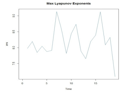
In the last decade there is a constantly growing interest in application of mathematics methods and econophysics methods to solve various problems concerning finance,economics,etc. Chaos and its application are importance for most of the current financial and economic phenomena. Financial markets can potentially provide financial long-term series which can be used in analysing and forecasting. Most recent studies,shows the existence of long and short-range correlations in the financial market and economic phenomena. For testing the existence of chaotic behaviour,Lyapunov's method is one of the best methods. In the current study time-series tests of Lyapunov's method were applied,among listed companies on Tehran stock exchange over a period from 2005 to 2015. The obtained findings prove the existence multifractality process in the evolution of time series stock price.
Citation: Mohammad Reza Abbaszadeh, Mehdi Jabbari Nooghabi, Mohammad Mahdi Rounaghi. Using Lyapunov's method for analysing of chaotic behaviour on financial time series data: a case study on Tehran stock exchange[J]. National Accounting Review, 2020, 2(3): 297-308. doi: 10.3934/NAR.2020017
In the last decade there is a constantly growing interest in application of mathematics methods and econophysics methods to solve various problems concerning finance,economics,etc. Chaos and its application are importance for most of the current financial and economic phenomena. Financial markets can potentially provide financial long-term series which can be used in analysing and forecasting. Most recent studies,shows the existence of long and short-range correlations in the financial market and economic phenomena. For testing the existence of chaotic behaviour,Lyapunov's method is one of the best methods. In the current study time-series tests of Lyapunov's method were applied,among listed companies on Tehran stock exchange over a period from 2005 to 2015. The obtained findings prove the existence multifractality process in the evolution of time series stock price.

| [1] | Arnold L, Doyle MM, Sri Namachchivaya N (1997) Small noise expansion of moment Lyapunov exponents for two-dimensional systems. Dyn Stab Syst 12: 187-211. |
| [2] | Dai M, Hou J, Gao J, et al. (2016) Mixed multifractal analysis of China and US stock index series. Chaos Soliton Fract 87: 268-275. |
| [3] | De Luca G, Loperfido N (2004) A Skew-in-Mean GARCH Model for Financial Returns, In Skew-Elliptical Distributions and Their Applications: A Journey Beyond Normality, CRC Press, 205-222. |
| [4] | De Luca G, Loperfido N (2015) Modelling Multivariate Skewness in Financial Returns: a SGARCH Approach. Eur J Financ 21: 1113-1131. |
| [5] | Engle RF (1982) Autoregressive conditional heteroskedasticity with estimates of the variance of U.K. inflation. Econometrica 50: 987-1008. |
| [6] | Fernandez A, Swanson NR (2017) Further Evidence on the Usefulness of Real-Time Datasets for Economic Forecasting. Quant Financ Econ 1: 2-25. |
| [7] | Foley DK (2016) Can economics be a physical science? Eur Phys J-Spec Top 225: 3171-3178. |
| [8] | Ghadiri Moghadam A, Jabbari Nooghabi M, Rounaghi MM, et al. (2014) Chaos Process Testing (Time-Series in The Frequency Domain) in Predicting Stock Returns in Tehran Stock Exchange. Indian J Sci Res 4: 202-210. |
| [9] | Gomez IS (2017) Lyapunov exponents and poles in a non Hermitian dynamics. Chas Soliton Fract 99: 155-161. |
| [10] | Gupta P, Batra SS, Jayadeva (2017) Sparse Short-Term Time Series Forecasting Models via Minimum Model Complexity. Neurocomputing 243: 1-11. |
| [11] | Gyamerah SA (2019) Modelling the volatility of Bitcoin returns using GARCH models. Quant Financ Econ 3: 739-753. |
| [12] | Ibarra-Valdez C, Alvarez J, Alvarez-Ramirez J (2016) Randomness confidence bands of fractal scaling exponents for financial price returns. Chaos Soliton Fract 83: 119-124. |
| [13] | Jahanshahi H, Yousefpour A, Wei Z, et al. (2019) A financial hyperchaotic system with coexisting attractors: Dynamic investigation, entropy analysis, control and synchronization. Chaos Soliton Fract 126: 66-77. |
| [14] | Kaplan DT, Glass L (1992) Direct test for determinism in a time series. Phys Rev Lett 68: 427-430. |
| [15] | Lahmiri S (2017a) A study on chaos in crude oil markets before and after 2008 international financial crisis. Physica A 466: 389-395. |
| [16] | Lahmiri S (2017b) Investigating existence of chaos in short and long term dynamics of Moroccan exchange rates. Physica A 465: 655-661. |
| [17] | Lahmiri S, Uddin GS, Bekiros S (2017) Nonlinear dynamics of equity, currency and commodity markets in the aftermath of the global financial crisis. Chaos Soliton Fract 103: 342-346. |
| [18] | Li DY, Nishimura Y, Men M (2014) Fractal markets: Liquidity and investors on different time horizons. Physica A 407: 144-151. |
| [19] | Li R, Wang J (2017) Symbolic complexity of volatility duration and volatility difference component on voter financial dynamics. Digit Signal Process 63: 56-71. |
| [20] | Madaleno M, Vieira E (2018) Volatility analysis of returns and risk: Family versus nonfamily firms. Quant Financ Econ 2: 348-372. |
| [21] | Mantegna RN, Stanley HE (1996) Turbulence and financial markets. Nature 383: 587-588. |
| [22] | Mantegna RN, Palagyi Z, Stanley HE (1999) Applications of statistical mechanics to finance. Physica A 274: 216-221. |
| [23] | Mastroeni L, Vellucci P, Naldi M (2018) Co-existence of stochastic andchaotic behaviour in the copper price time series. Resour Policy 58:295-302. |
| [24] | Mastroeni L, Vellucci P, Naldi M (2019) A reappraisal of the chaoticparadigm for energy commodity prices. Energ Econ 82: 167-178. |
| [25] | Moradi M, Jabbari Nooghabi M, Rounaghi MM (2019) Investigation of fractal market hypothesis and forecasting time series stock returns for Tehran Stock Exchange and London Stock Exchange. Int J Financ Econ, 1-17. |
| [26] | Münnix M, Shimada T, Schä fer R (2012) Identifying states of a financial market. Sci Rep 2: 644-647. |
| [27] | Nair BB, Kumar PK, Sakthivel NR, et al. (2017) Clustering stock price time series data to generate stock trading recommendations: An empirical study. Expert Syst Appl 70: 20-36. |
| [28] | Niu H, Wang H (2013a) Complex dynamic behaviors of oriented percolation-based financial time series and Hang Seng index. Chaos Soliton Fract 52: 36-44. |
| [29] | Niu H, Wang H (2013b) Volatility clustering and long memory of financial time series and financial price model. Digit Signal Process 23: 489-498. |
| [30] | Ola MR, Jabbari Nooghabi M, Rounaghi MM (2014) Chaos Process Testing (Using Local Polynomial Approximation Model) in Predicting Stock Returns in Tehran Stock Exchange. Asian J Res Bank Financ 4: 100-109. |
| [31] | Peinke J, Parisi J, Parisi OE, et al. (1992) Encounter with Chaos, Springer-Verlag. |
| [32] | Podsiadlo M, Rybinski H (2016) Financial time series forecasting using rough sets with time-weighted rule voting. Expert Syst Appl 66: 219-233. |
| [33] | Rosini L, Shenai V (2020) Stock returns and calendar anomalies on the London Stock Exchange in the dynamic perspective of the Adaptive Market Hypothesis: A study of FTSE100 & FTSE250 indices over a ten year period. Quant Financ Econ 4: 121-147. |
| [34] | Rounaghi MM, Abbaszadeh MR, Arashi M (2015) Stock price forecasting for companies listed on Tehran stock exchange using multivariate adaptive regression splines model and semi-parametric splines technique. Physica A 438: 625-633. |
| [35] | Rounaghi MM, Nassir Zadeh F (2016) Investigation of market efficiency and Financial Stability between S & P 500 and London Stock Exchange: Monthly and yearly Forecasting of Time Series Stock Returns using ARMA model. Physica A 456: 10-21. |
| [36] | Rydber TH (2000) Realistic Statistical Modelling of Financial Data. Int Stat Rev 68: 233-258. |
| [37] | Salvino LW, Cawley R (1994) Smoothness implies determinism: a method to detect it in time series. Phys Rev Lett 73:1091-1094. |
| [38] | Shynkevich Y, McGinnity TM, Coleman SA, et al. (2017) Forecasting price movements using technical indicators: Investigating the impact of varying input window length. Neurocomputing 264: 71-88. |
| [39] | Su CH, Cheng CH (2016) A Hybrid Fuzzy Time Series Model Based on ANFIS and Integrated Nonlinear Feature Selection Method for Forecasting Stock. Neurocomputing 205: 264-273. |
| [40] | Sun Y, Wang X, Wu Q, et al. (2011) On stability analysis via Lyapunov exponents calculated based on radial basis function networks. Int J Control 84: 1326-1341. |
| [41] | Takaishi T (2017) Volatility estimation using a rational GARCH model. Quant Financ Econ 2: 127-136. |
| [42] | Wayland R, Bromley D, Pickett D, et al. (1993) Recog-nizing determinism in a time series. Phys Rev Lett 70: 580-582. |
| [43] | Wei LY (2016) A hybrid ANFIS model based on empirical mode decomposition for stock time series forecasting. Appl Soft Comput 42: 368-376. |
| [44] | Zahedi J, Rounaghi MM (2015) Application of artificial neural network models and principal component analysis method in predicting stock prices on Tehran Stock Exchange. Physica A 438: 178-187. |
| [45] | Zhong X, Enke D (2017) A Comprehensive Cluster and Classification Mining Procedure for Daily Stock Market Return Forecasting. Neurocomputing 267: 152-168. |
Figures(2) / Tables(1)

Mohammad Reza Abbaszadeh, Mehdi Jabbari Nooghabi, Mohammad Mahdi Rounaghi. Using Lyapunov's method for analysing of chaotic behaviour on financial time series data: a case study on Tehran stock exchange[J]. National Accounting Review, 2020, 2(3): 297-308. doi: 10.3934/NAR.2020017


 DownLoad: