Beyond “#endpjparalysis”, tackling sedentary behaviour in health care

Sebastien FM Chastin; Juliet A Harvey; Philippa M Dall; Lianne McInally; Alexandra Mavroeidi; Dawn A Skelton; Sebastien FM Chastin; Juliet A Harvey; Philippa M Dall; Lianne McInally; Alexandra Mavroeidi; Dawn A Skelton

doi:10.3934/medsci.2019.1.67

AIMS Medical Science

2019, Volume 6, Issue 1:67-75. doi: 10.3934/medsci.2019.1.67

Previous Article Next Article

Editorial Special Issues

Beyond “#endpjparalysis”, tackling sedentary behaviour in health care

1.
Centre for Living, School of Health and Life Sciences, Glasgow Caledonian University, Glasgow, Scotland, UK
2.
Department of Sport and Movement Science, Ghent University, Ghent, Belgium
3.
NHS Greater Glasgow & Clyde, Glasgow, UK
4.
Falls Service, NHS Lanarkshire, Glasgow, UK

Received: 27 June 2018 Accepted: 31 January 2019 Published: 02 February 2019

Abstract
Full Text(HTML)
Download PDF

Reducing Sedentary Behaviour after hospitalization starts with reducing sedentary behaviour whilst in hospital. Although we have eradicated immobilisation as a therapeutic tool due to its potent detrimental effects, it is still in systemic use within health care systems and hospitals. Evidence shows that when in hospital, patients spend most of their time sedentary. In this editorial, we explore the determinants of, and a system-based approach to, reducing sedentary behaviour in health care.
- sitting,
- physical activity,
- ageing,
- inactivity
Citation: Sebastien FM Chastin, Juliet A Harvey, Philippa M Dall, Lianne McInally, Alexandra Mavroeidi, Dawn A Skelton. Beyond “#endpjparalysis”, tackling sedentary behaviour in health care[J]. AIMS Medical Science, 2019, 6(1): 67-75. doi: 10.3934/medsci.2019.1.67

Related Papers:

Abstract

Reducing Sedentary Behaviour after hospitalization starts with reducing sedentary behaviour whilst in hospital. Although we have eradicated immobilisation as a therapeutic tool due to its potent detrimental effects, it is still in systemic use within health care systems and hospitals. Evidence shows that when in hospital, patients spend most of their time sedentary. In this editorial, we explore the determinants of, and a system-based approach to, reducing sedentary behaviour in health care.

Conflict of interest

The authors declare no conflict of interest.

References

[1]	Baldwin C, van Kessel G, Phillips A, et al. (2017) Accelerometry shows inpatients with acute medical or surgical conditions spend little time upright and are highly sedentary: Systematic review. Phys Ther 97: 1044–1065.
[2]	Tremblay MS, Aubert S, Barnes JD, et al. (2017) Sedentary Behavior Research Network (SBRN) - Terminology Consensus Project process and outcome. Int J Behav Nutr Phys Act 14: 75. doi: 10.1186/s12966-017-0525-8
[3]	Chastin SFM, Scwartz U, Skelton DA (2013) Development of a consensus taxonomy of sedentary behaviors (SIT): Report of Delphi Round 1. PLoS One 8: e82313. doi: 10.1371/journal.pone.0082313
[4]	Grant PM, Granat MH, Thow MK, et al. (2010) Analyzing free-living physical activity of older adults in different environments using body-worn activity monitors. J Aging Phys Act 18: 171–184. doi: 10.1123/japa.18.2.171
[5]	Sjöholm A, Skarin M, Churilov L, et al. (2014) Sedentary behaviour and physical activity of people with stroke in rehabilitation hospitals. Stroke Res Treat 2014: 591897.
[6]	Karbiener M, Pisani DF, Frontini A, et al. (2014) MicroRNA-26 family is required for human adipogenesis and drives characteristics of brown adipocytes. Stem Cells 32: 1578–1590. doi: 10.1002/stem.1603
[7]	Taraldsen K, Thingstad P, Sletvold O, et al. (2015) The long-term effect of being treated in a geriatric ward compared to an orthopaedic ward on six measures of free-living physical behavior 4 and 12 months after a hip fracture - A randomised controlled trial. BMC Geriatr 15: 160. doi: 10.1186/s12877-015-0153-6
[8]	Egerton T, Maxwell DJ, Granat MH (2006) Mobility activity of stroke patients during inpatient rehabilitation. Hong Kong Physiother J 24: 8–15. doi: 10.1016/S1013-7025(07)70003-9
[9]	Harvey JA, Chastin SFM, Skelton DA (2018) What happened to my legs when I broke my arm? Aims Med Sci 5: 252–258. doi: 10.3934/medsci.2018.3.252
[10]	Chastin SFM, Egerton T, Leask C, et al. (2015) Meta-analysis of the relationship between breaks in sedentary behavior and cardiometabolic health. Obesity 23: 1800–1810. doi: 10.1002/oby.21180
[11]	Matthews CE, Keadle SK, Troiano RP, et al. (2016) Accelerometer-measured dose-response for physical activity, sedentary time, and mortality in US adults. Am J Clin Nutr 104: 1424–1432. doi: 10.3945/ajcn.116.135129
[12]	Biswas A, Oh PI, Faulkner GE, et al. (2015) Sedentary time and its association with risk for disease incidence, mortality, and hospitalization in adults: A systematic review and meta-analysis. Ann Intern Med 162: 123–132. doi: 10.7326/M14-1651
[13]	Ekegren CL, Beck B, Climie RE, et al. (2018) Physical activity and sedentary behavior subsequent to serious orthopedic injury: A systematic review. Arch Phys Med Rehabil 99: 164–177. doi: 10.1016/j.apmr.2017.05.014
[14]	Zusman EZ, Dawes MG, Edwards N, et al. (2018) A systematic review of evidence for older adults' sedentary behavior and physical activity after hip fracture. Clin Rehabil 32: 679–691. doi: 10.1177/0269215517741665
[15]	Tieges Z, Mead G, Allerhand M, et al. (2015) Sedentary behavior in the first year after stroke: A longitudinal cohort study with objective measures. Arch Phys Med Rehabil 96: 15–23. doi: 10.1016/j.apmr.2014.08.015
[16]	Kronborg L, Bandholm T, Palm H, et al. (2016) Physical activity in the acute ward following hip fracture surgery is associated with less fear of falling. J Aging Phys Act 24: 525–532. doi: 10.1123/japa.2015-0071
[17]	Krumholz HM (2013) Post-hospital syndrome-an acquired, transient condition of generalized risk. N Engl J Med 368: 100–102. doi: 10.1056/NEJMp1212324
[18]	Hodgson CL, Capell E, Tipping CJ (2018) Early mobilization of patients in intensive care: Organization, communication and safety factors that influence translation into clinical practice. Crit Care 22: 77. doi: 10.1186/s13054-018-1998-9
[19]	Dogra S, Ashe MC, Biddle SJH, et al. (2017) Sedentary time in older men and women: an international consensus statement and research priorities. Br J Sports Med 51: 1526–1532. doi: 10.1136/bjsports-2016-097209
[20]	Kortebein P (2009) Rehabilitation for hospital-associated deconditioning. Am J Phys Med Rehabil 88: 66–77. doi: 10.1097/PHM.0b013e3181838f70
[21]	Skelton D, Van Wijck F, Grant M, et al. (2014) Are physiotherapists contributing to patient harm? Are your patients FIT TO SIT? Agility 20.
[22]	Boltz M, Resnick B, Capezuti E, et al. (2014) Activity restriction vs. self-direction: hospitalised older adults' response to fear of falling. Int J Older People Nurs 9: 44–53.
[23]	Resnick B, Galik E, Wells CL, et al. (2015) Optimizing physical activity among older adults post trauma: Overcoming system and patient challenges. Int J Orthop Trauma Nurs 19: 194–206. doi: 10.1016/j.ijotn.2015.03.007
[24]	Owen N, Sugiyama T, Eakin EE, et al. (2011) Adults' sedentary behavior determinants and interventions. Am J Prev Med 41: 189–196. doi: 10.1016/j.amepre.2011.05.013
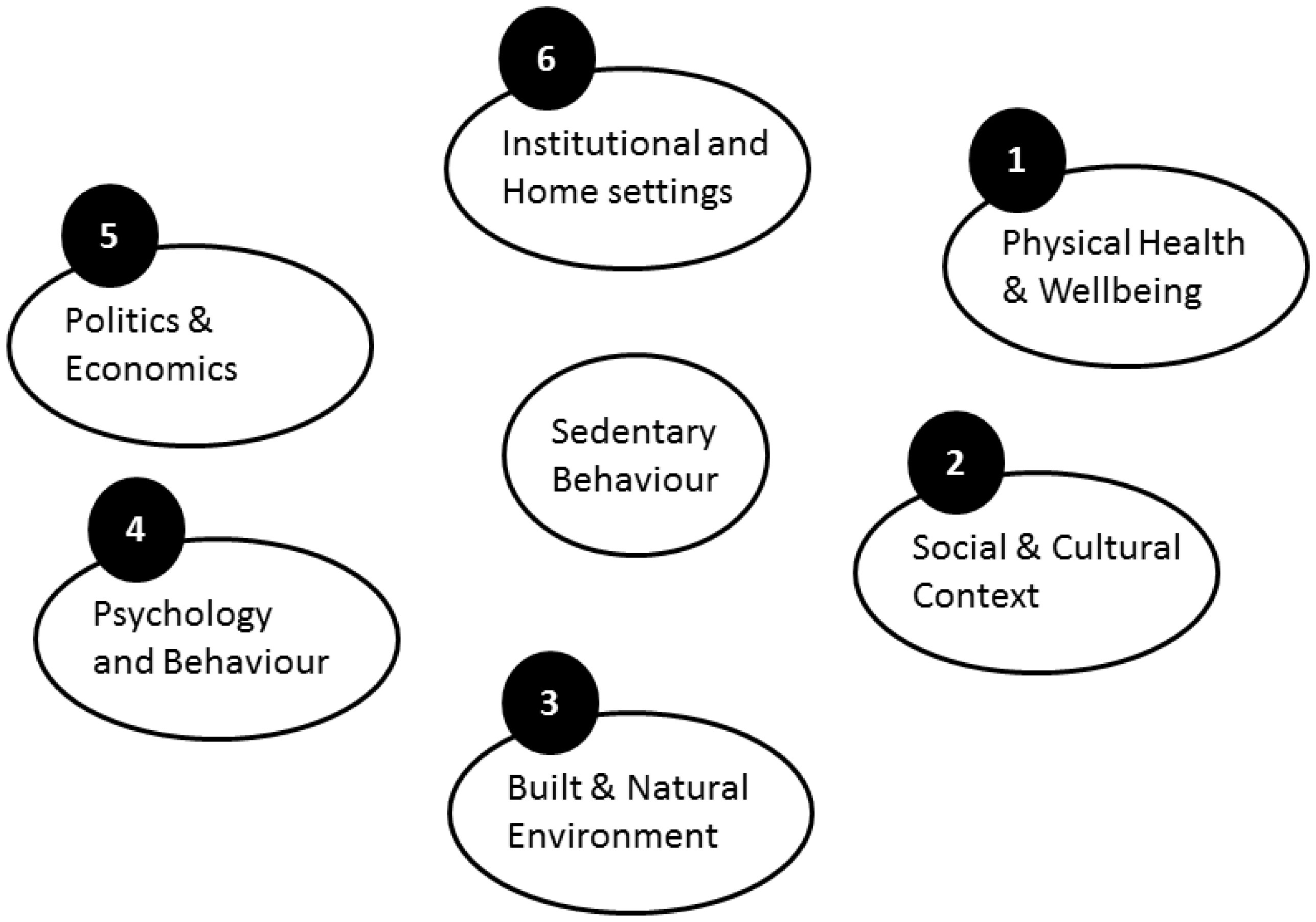
[25]	Chastin SFM, De Craemer M, Lien N, et al. (2016) The SOS-framework (Systems of Sedentary behaviours): An international transdisciplinary consensus framework for the study of determinants, research priorities and policy on sedentary behaviour across the life course: A DEDIPAC-study. Int J Behav Nutr Phys Act 13: 83. doi: 10.1186/s12966-016-0409-3
[26]	Organisation for Economic and Cooperation Development (2009) Applications of Complexity Science for Public Policy.
[27]	Finegood DT, Karanfil O, Matteson CL (2008) Getting from analysis to action: framing obesity research, policy and practice with a solution-oriented complex systems lens. Healthc Pap 9: 36–41. doi: 10.12927/hcpap.2008.20184
[28]	Greenhalgh T, Jackson C, Shaw S, et al. (2016) Achieving research impact through co-creation in community-based health services: Literature review and case study. Milbank Q 94: 392–429. doi: 10.1111/1468-0009.12197
[29]	Boltz M, Resnick B, Capezuti E, et al. (2012) Functional decline in hospitalized older adults: Can nursing make a difference? Geriatr Nurs 33: 272–279. doi: 10.1016/j.gerinurse.2012.01.008
[30]	Langley GJ, Moen R, Nolan KM, et al. (2009) The improvement guide: A practical approach to enhancing organizational performance. 2nd Edition.
[31]	Hartley PJ, Keevil VL, Alushi L, et al. (2017) Earlier physical therapy input is associated with a reduced length of hospital stay and reduced care needs on discharge in frail older inpatients: An observational study. J Geriatr Phys Ther doi: 10.1519/JPT.0000000000000134.
[32]	Dall P, Coulter EH, Fitzsimons C, et al. (2017) The TAxonomy of Self-reported Sedentary behaviour Tools (TASST) framework for development, comparison and evaluation of self-report tools: Content analysis and systematic review. BMJ Open 7: e013844. doi: 10.1136/bmjopen-2016-013844
[33]	Chastin SFM, Dontje ML, Skelton DA, et al. (2018) Systematic comparative validation of self-report measures of sedentary time against an objective measure of postural sitting (activPAL). Int J Behav Nutr Phys Act 15: 21. doi: 10.1186/s12966-018-0652-x
[34]	Crouter SE, Clowers KG, Bassett DR Jr (2006) A novel method for using accelerometer data to predict energy expenditure. J Appl Physiol 100: 1324–1331. doi: 10.1152/japplphysiol.00818.2005
[35]	Sellers C, Dall P, Grant M, et al. (2016) Validity and reliability of the activPAL3 for measuring posture and stepping in adults and young people. Gait Posture 43: 42–47. doi: 10.1016/j.gaitpost.2015.10.020
[36]	Fortune E, Lugade VA, Amin S, et al. (2015) Step detection using multi- versus single tri-axial accelerometer-based systems. Physiol Meas 36: 2519–2535. doi: 10.1088/0967-3334/36/12/2519
[37]	Cook DJ, Thompson JE, Prinsen SK, et al. (2013) Functional recovery in the elderly after major surgery: Assessment of mobility recovery using wireless technology. Ann Thorac Surg 96: 1057–1061. doi: 10.1016/j.athoracsur.2013.05.092
[38]	Ryan CG, Grant PM, Tigbe WW, et al. (2006) The validity and reliability of a novel activity monitor as a measure of walking. Br J Sports Med 40: 779–784. doi: 10.1136/bjsm.2006.027276
[39]	Loveday A, Sherar LB, Sanders JP, et al. (2015) Technologies that assess the location of physical activity and sedentary behavior: A systematic review. J Med Internet Res 17: e192. doi: 10.2196/jmir.4761

Reader Comments

your name:*

Email:*
© 2019 the Author(s), licensee AIMS Press. This is an open access article distributed under the terms of the Creative Commons Attribution License (http://creativecommons.org/licenses/by/4.0)