The impact of immune cell interactions on virus quasi-species formation

Ali Moussaoui; Vitaly Volpert; Ali Moussaoui; Vitaly Volpert

doi:10.3934/mbe.2024331

Mathematical Biosciences and Engineering

2024, Volume 21, Issue 11: 7530-7553. doi: 10.3934/mbe.2024331

Previous Article Next Article

Research article Special Issues

The impact of immune cell interactions on virus quasi-species formation

Ali Moussaoui ^{1
,
,},
Vitaly Volpert ^2,3,4

1.
Laboratoire d'Analyse Non Linéaire et Mathématiques Appliquées, Department of Mathematics, Faculty of Science, University of Tlemcen, 13000, Algeria
2.
Institut Camille Jordan, UMR 5208 CNRS, University Lyon 1, Villeurbanne 69622, France
3.
Peoples' Friendship University of Russia (RUDN University)
4.
Miklukho-Maklaya St, Moscow 117198, Russian Federation

Received: 27 July 2024 Revised: 18 October 2024 Accepted: 28 October 2024 Published: 11 November 2024

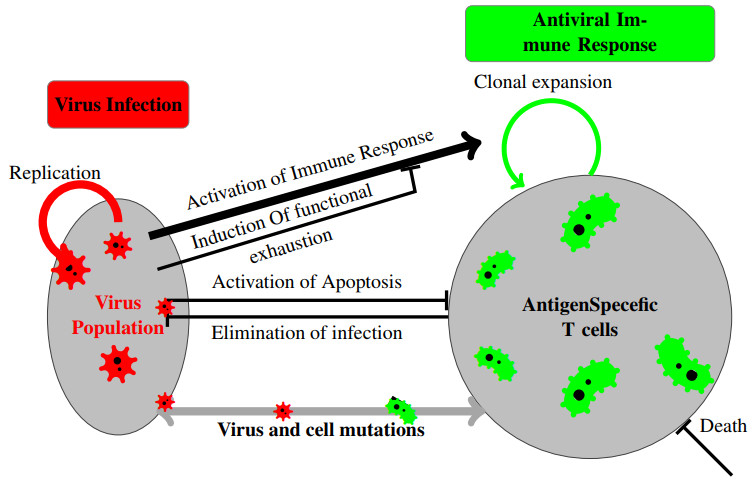
The process of viral infection spreading in tissues was influenced by various factors, including virus replication within host cells, transportation, and the immune response. Reaction-diffusion systems provided a suitable framework for examining this process. In this work, we studied a nonlocal reaction-diffusion system of equations that modeled the distribution of viruses based on their genotypes and their interaction with the immune response. It was shown that the infection may persist at a certain level alongside a chronic immune response, exhibiting spatially uniform or oscillatory behavior. Finally, the immune cells may become entirely depleted, leading to a high viral load persisting in the tissue. Numerical simulations were employed to elucidate the nonlinear dynamics and pattern formation inherent in the nonlocal model.
- virus density distribution,
- nonlocal interaction,
- genotype space,
- immune response,
- reaction-diffusion model
Citation: Ali Moussaoui, Vitaly Volpert. The impact of immune cell interactions on virus quasi-species formation[J]. Mathematical Biosciences and Engineering, 2024, 21(11): 7530-7553. doi: 10.3934/mbe.2024331

Related Papers:

Abstract

The process of viral infection spreading in tissues was influenced by various factors, including virus replication within host cells, transportation, and the immune response. Reaction-diffusion systems provided a suitable framework for examining this process. In this work, we studied a nonlocal reaction-diffusion system of equations that modeled the distribution of viruses based on their genotypes and their interaction with the immune response. It was shown that the infection may persist at a certain level alongside a chronic immune response, exhibiting spatially uniform or oscillatory behavior. Finally, the immune cells may become entirely depleted, leading to a high viral load persisting in the tissue. Numerical simulations were employed to elucidate the nonlinear dynamics and pattern formation inherent in the nonlocal model.

References

[1]	P. Auger, A. Moussaoui, On the threshold of release of confinement in an epidemic SEIR model taking into account the protective effect of mask, Bull. Math. Biol., 83 (2021), 25. https://doi.org/10.1007/s11538-021-00858-8 doi: 10.1007/s11538-021-00858-8
[2]	A. Moussaoui, M. Meziane, On the date of the epidemic peak, Math. Biosci. Eng., 21 (2024), 2835–2855. https://doi.org/10.3934/mbe.2024126 doi: 10.3934/mbe.2024126
[3]	A. Moussaoui, E. H. Zerga, Transmission dynamics of COVID-19 in Algeria: The impact of physical distancing and face masks, AIMS Public Health, 7 (2020), 816–827. https://doi.org/10.3934/publichealth.2020063 doi: 10.3934/publichealth.2020063
[4]	A. Moussaoui, P. Auger, Prediction of confinement effects on the number of COVID-19 outbreaks in Algeria, Math. Model. Nat. Phenom., 15 (2020), 37. https://doi.org/10.1051/mmnp/2020028 doi: 10.1051/mmnp/2020028
[5]	A. Moussaoui, Estimating the final size relation for the SIR discrete epidemic model under intervention, Nonlinear Stud., 31 (2024), 1. https://nonlinearstudies.com/index.php/nonlinear/article/view/3221
[6]	T. Nguyen-Huu, P. Auger, A. Moussaoui, On incidence-dependent management strategies against an SEIRS epidemic: Extinction of the epidemic using Allee effect, Mathematics, 11 (2023), 2822. https://doi.org/10.3390/math11132822 doi: 10.3390/math11132822
[7]	G. Bocharov, A. Meyerhans, N. Bessonov, S. Trofimchuk, V. Volpert, Interplay between reaction and diffusion processes in governing the dynamics of virus infections, J. Theor. Biol., 457 (2018), 221–236. https://doi.org/10.1016/j.jtbi.2018.08.036. doi: 10.1016/j.jtbi.2018.08.036
[8]	J. N. Mandl, P. Torabi-Parizi, R. N. Germain, Visualization and dynamic analysis of host-pathogen interactions, Curr. Opin. Immunol., 29 (2014), 8–15. https://doi.org/10.1016/j.coi.2014.03.002 doi: 10.1016/j.coi.2014.03.002
[9]	X. Sewald, N. Motamedi, W. Mothes, Viruses exploit the tissue physiology of the host to spread in vivo, Curr. Opin. Cell Biol., 41 (2016), 81–90. https://doi.org/10.1016/j.ceb.2016.04.008 doi: 10.1016/j.ceb.2016.04.008
[10]	C. K. Biebricher, M. Eigen, What is a quasispecies?, Curr. Top Microbiol. Immunol., 299 (2006), 1–31.
[11]	E. Domingo, J. Sheldon, C. Perales, Viral quasispecies evolution, Microbiol. Mol. Biol. Rev., 76 (2012), 159–216. https://doi.org/10.1128/mmbr.05023-11 doi: 10.1128/mmbr.05023-11
[12]	M. Nowak, R. M. May, Virus Dynamics, in Mathematical Principles of Immunology and Virology, Oxford University Press, 2000.
[13]	M. Meziane, A. Moussaoui, V. Volpert, On a two-strain epidemic model involving delay equations, Math. Biosci. Eng., 20 (2023), 20683–20711. https://doi.org/10.3934/mbe.2023915 doi: 10.3934/mbe.2023915
[14]	N. Bessonov, G. Bocharov, A. Meyerhans, V. Popov, V. Volpert, Existence and dynamics of strains in a nonlocal reaction-diffusion model of viral evolution, SIAM J. Appl. Math., 81 (2021), 107–128, https://doi.org/10.1137/19M1282234 doi: 10.1137/19M1282234
[15]	M. Kimura, Diffusion models in population genetics, J. Appl. Probab., 1 (1964), 177–232. https://doi.org/10.2307/3211856 doi: 10.2307/3211856
[16]	A. Sasaki, Evolution of antigen drift/switching: continuously evading pathogens, J. Theor. Biol., 163 (1994), 291–308. https://doi.org/10.1006/jtbi.1994.1110 doi: 10.1006/jtbi.1994.1110
[17]	N. Bessonov, G. A. Bocharov, C. Leon, V. Popov, V. Volpert, Genotype-dependent virus distribution and competition of virus strains, Math. Mech. Complex Syst., 8 (2020), 101–126. https://doi.org/10.2140/memocs.2020.8.101 doi: 10.2140/memocs.2020.8.101
[18]	A. Moussaoui, V. Volpert, The influence of immune cells on the existence of virus quasi-species, Math. Biosci. Eng., 20 (2023), 15942–15961. https://doi.org/10.3934/mbe.2023710 doi: 10.3934/mbe.2023710
[19]	G. Bocharov, A. Meyerhans, N. Bessonov, S. Trofimchuk, V. Volpert, Modelling the dynamics of virus infection and immune response in space and time, Int. J. Parallel, Emergent Distrib. Syst., 34 (2019), 341–355. https://doi.org/10.1080/17445760.2017.1363203 doi: 10.1080/17445760.2017.1363203
[20]	A. Mozokhina, L. A. Mahiout, V. Volpert, Modeling of viral infection with inflammation, Mathematics, 11 (2023), 4095. https://doi.org/10.3390/math11194095 doi: 10.3390/math11194095
[21]	V. Volpert, Elliptic Partial Differential Equations, Volume 2: Reaction-Diffusion Equations, Villeurbanne: Birkhäuser, 2014.
[22]	A. Volpert, V. Volpert, Spectrum of elliptic operators and stability of travelling waves, Asymptotic Anal., 23 (2000), 111–134.
[23]	B. Anderson, J. Jackson, M. Sitharam, Descartes rule of signs revisited, Am. Math. Mon., 105 (1998), 447–151. https://doi.org/10.1080/00029890.1998.12004907 doi: 10.1080/00029890.1998.12004907
[24]	J. D. Murray, Mathematical Biology II, Heidelberg, Springer-Verlag, 2002.
[25]	R. S. Strichartz, A Guide to Distribution Theory and Fourier Transforms, World Scientific, Singapour, 2003.
[26]	S. Genieys, V. Volpert, P. Auger, Pattern and waves for a model in population dynamics with nonlocal consumption of resources, Math. Model. Nat. Phenom., 1 (2006), 63–80. https://doi.org/10.1051/mmnp:2006004 doi: 10.1051/mmnp:2006004
[27]	B. L Segal, V. Volpert, A. Bayliss, Pattern formation in a model of competing populations with nonlocal interactions, Phys. D: Nonlinear Phenom., 253 (2013), 12–23. https://doi.org/10.1016/j.physd.2013.02.006 doi: 10.1016/j.physd.2013.02.006
[28]	N. Bessonov, N. Reinberg, M. Banerjee, V. Volpert, The origin of species by means of mathematical modelling, Acta Biotheor., 66 (2018), 333–344. https://doi.org/10.1007/s10441-018-9328-9 doi: 10.1007/s10441-018-9328-9
[29]	N. Bessonov, D. Neverova, V. Popov, V. Volpert, Emergence and competition of virus variants in respiratory viral infections, Front. Immunol., 13 (2023), 945228. https://doi.org/10.3389/fimmu.2022.945228. doi: 10.3389/fimmu.2022.945228

Reader Comments

Your name:*

Email:*
© 2024 the Author(s), licensee AIMS Press. This is an open access article distributed under the terms of the Creative Commons Attribution License (http://creativecommons.org/licenses/by/4.0)