Asymptotic behavior of the solutions for a stochastic SIRS model with information intervention

Tingting Ding; Tongqian Zhang; Tingting Ding; Tongqian Zhang

doi:10.3934/mbe.2022327

Mathematical Biosciences and Engineering

2022, Volume 19, Issue 7: 6940-6961. doi: 10.3934/mbe.2022327

Previous Article Next Article

Research article Special Issues

Asymptotic behavior of the solutions for a stochastic SIRS model with information intervention

Tingting Ding ,
Tongqian Zhang ^,

College of Mathematics and Systems Science, Shandong University of Science and Technology, Qingdao 266590, China

Academic Editor: Sanling Yuan

Received: 09 April 2022 Revised: 26 April 2022 Accepted: 04 May 2022 Published: 09 May 2022

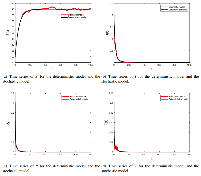
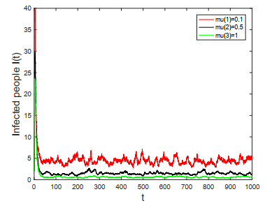
In this paper, a stochastic SIRS epidemic model with information intervention is considered. By constructing an appropriate Lyapunov function, the asymptotic behavior of the solutions for the proposed model around the equilibria of the deterministic model is investigated. We show the average in time of the second moment of the solutions of the stochastic system is bounded for a relatively small noise. Furthermore, we find that information interaction response rate plays an active role in disease control, and as the intensity of the response increases, the number of infected population decreases, which is beneficial for disease control.

Keywords:

Citation: Tingting Ding, Tongqian Zhang. Asymptotic behavior of the solutions for a stochastic SIRS model with information intervention[J]. Mathematical Biosciences and Engineering, 2022, 19(7): 6940-6961. doi: 10.3934/mbe.2022327

Related Papers:

[1]	Takeshi Miyama, Sung-mok Jung, Katsuma Hayashi, Asami Anzai, Ryo Kinoshita, Tetsuro Kobayashi, Natalie M. Linton, Ayako Suzuki, Yichi Yang, Baoyin Yuan, Taishi Kayano, Andrei R. Akhmetzhanov, Hiroshi Nishiura . Phenomenological and mechanistic models for predicting early transmission data of COVID-19. Mathematical Biosciences and Engineering, 2022, 19(2): 2043-2055. doi: 10.3934/mbe.2022096
[2]	Sanling Yuan, Xuehui Ji, Huaiping Zhu . Asymptotic behavior of a delayed stochastic logistic model with impulsive perturbations. Mathematical Biosciences and Engineering, 2017, 14(5&6): 1477-1498. doi: 10.3934/mbe.2017077
[3]	Kangbo Bao, Qimin Zhang, Xining Li . A model of HBV infection with intervention strategies: dynamics analysis and numerical simulations. Mathematical Biosciences and Engineering, 2019, 16(4): 2562-2586. doi: 10.3934/mbe.2019129
[4]	Yu Zhu, Liang Wang, Zhipeng Qiu . Threshold behaviour of a stochastic SIRS $ \mathrm {L\acute{e}vy} $ jump model with saturated incidence and vaccination. Mathematical Biosciences and Engineering, 2023, 20(1): 1402-1419. doi: 10.3934/mbe.2023063
[5]	Qingshan Yang, Xuerong Mao . Stochastic dynamics of SIRS epidemic models withrandom perturbation. Mathematical Biosciences and Engineering, 2014, 11(4): 1003-1025. doi: 10.3934/mbe.2014.11.1003
[6]	Zhongwei Cao, Jian Zhang, Huishuang Su, Li Zu . Threshold dynamics of a stochastic general SIRS epidemic model with migration. Mathematical Biosciences and Engineering, 2023, 20(6): 11212-11237. doi: 10.3934/mbe.2023497
[7]	Tingting Yu, Sanling Yuan . Dynamics of a stochastic turbidostat model with sampled and delayed measurements. Mathematical Biosciences and Engineering, 2023, 20(4): 6215-6236. doi: 10.3934/mbe.2023268
[8]	Cruz Vargas-De-León, Alberto d'Onofrio . Global stability of infectious disease models with contact rate as a function of prevalence index. Mathematical Biosciences and Engineering, 2017, 14(4): 1019-1033. doi: 10.3934/mbe.2017053
[9]	Ariel Cintrón-Arias, Carlos Castillo-Chávez, Luís M. A. Bettencourt, Alun L. Lloyd, H. T. Banks . The estimation of the effective reproductive number from disease outbreak data. Mathematical Biosciences and Engineering, 2009, 6(2): 261-282. doi: 10.3934/mbe.2009.6.261
[10]	Yanyan Du, Ting Kang, Qimin Zhang . Asymptotic behavior of a stochastic delayed avian influenza model with saturated incidence rate. Mathematical Biosciences and Engineering, 2020, 17(5): 5341-5368. doi: 10.3934/mbe.2020289

Abstract

1. Introduction

Infectious diseases seriously affect human's daily life and cause great losses to society and economy. It is one of the biggest public enemies threatening human life and health. According to the World Health Organization (WHO) Report, 2.6 million people died from lower respiratory tract infections worldwide in 2019 ^[1], and 10 million people were diagnosed with tuberculosis and 1.4 million people died of tuberculosis^[2]. Severe Acute Respiratory Syndrome (SARS) caused approximately USfanxiexian_myfh60 billion in losses to Asian countries in 2003^[3].There are more than 354 million people suffering from chronic hepatitis in the world, with an average of more than 8000 new hepatitis B and C patients every day, and more than 1 million deaths due to advanced liver disease and liver cancer each year^[4]. And the sudden outbreak of COVID-19 in early 2020 brought a catastrophe to humanity. As of October 3, 2021, the cumulative number of confirmed cases reported globally exceeded 234 million, and the cumulative death toll was just under 4.8 million^[5].

In recent decades, infectious disease dynamics models have become an effective tool for people to understand the spread and evolution of various infectious diseases^{[6,7,8,9,10,11,12]}. These models have played an important role in the prevention and control of infectious diseases^[10]. People usually adopt drug intervention (vaccination and drug treatment) to prevent and control the spread of infectious diseases, which has a good effect on the long-term control of infectious diseases. However, in recent years, researchers have found that in the absence of drug control, control through information plays a crucial role in the initial stages of the spread of infectious diseases. During the spread of an infectious disease, individual behaviors change in response to various infectious disease information. Such behavioral changes play an important role in the spread of emergent infectious diseases. Because after obtaining information on infectious diseases, people will try to reduce the possibility of infection by reducing gatherings, wearing masks, maintaining indoor ventilation, and strengthening disinfection of daily necessities to protect themselves. Therefore, although changes in personal behavior cannot eradicate infectious diseases, they can effectively delay the peak period of infectious disease outbreaks and reduce their severity ^[13,14,15]. It seems that the combined use of drug intervention and information intervention is better than a single intervention in controlling the spread of infectious diseases^[14], and many researchers have noticed the role of information intervention in controlling the spread of infectious diseases^[16,17,18].

Information control as a means of intervention can be spread through educational campaigns, the media, or the population itself through social activities^[14]. Researchers considered different methods to incorporate the impact of infectious disease information into the mathematical model of infectious diseases. The impact of media coverage on disease transmission can be accounted by considering a correction in the incidence rate with a saturated function of infective individuals in ^{[19,20,21,22,23,24,25,26]}. Considering the impact of disease epidemic information on individuals' behavioral responses, and the dissemination of such disease information through various media, including television, newspapers, social activities, and positive education programs by the government and local organizations, Anuj Kumar et al.^[14] established a model as follows,

$\begin{equation} \left\{\begin{array}{l} {\frac{dS(t)}{dt} = \Lambda-\mu S-\beta SI-\mu_{1}mZS+\delta_{0}R,}\\ {\frac{dI(t)}{dt} = \beta SI-(\mu+\delta+\gamma)I,}\\ {\frac{dR(t)}{dt} = \gamma I+\mu_{1}mZS-(\mu+\delta_{0})R,}\\ {\frac{dZ(t)}{dt} = \frac{aI}{1+bI}-a_{0}Z,} \end{array} \right. \end{equation}$

(1.1)

where $S(t)$ , $I(t)$ and $R(t)$ is the numbers of susceptible, infected, and recovered, respectively. $Z(t)$ represents the density of information. For the biological significance of all parameters, please refer to Anuj Kumar et al.^[14]. For model (1.1), Anuj Kumar et al.^[14] difined the basic reproductive number $R_{0} = \frac{\beta\Lambda}{\mu(\mu+\delta+\gamma)},$ and discussed the globally asymptotically stability of the equilibriua. The authors proved that if $R_{0} < 1,$ model (1.1) has a unique globally asymptotically stable disease-free equilibrium $E_{0} = (S_{0}, 0, 0, 0) = (\frac{\Lambda}{\mu}, 0, 0, 0);$ if $R_{0} > 1,$ model (1.1) has a unique globally asymptotically stable endemic equilibrium $E^{*} = (S^{*}, I^{*}, R^{*}, Z^{*}).$

However, the above models are deterministic models, but the real life world is full of randomness (such as fluctuations, noise, earthquakes, tsunamis, etc.), so it is particularly important to consider the random factors in the process of disease transmission. The stochastic infectious disease models are more realistic and have more dynamic properties. In recent years, many scholars have paid great attention to the study of stochastic infectious disease models and have produced many good results^{[27,28,29,30,31,32,33]}. For example, Zhao et al. ^[34] and Liu et al. ^[35] have investigated a stochastic SIVS epidemic model and a SIS epidemic model with nonlinear saturation rates respectively. In the model, they assumed that the contact rate $\beta$ was perturbed by white noise and studied the extinction and persistence of the disease by constructing suitable Lyapunov functions. Zhou et al. ^[36] have considered a stochastic SIR epidemic model with a general nonlinear incidence rate, the stationary distribution of the solutions of the system under certain parameter constraints is obtained. Zhou et al.^[37] have established the threshold dynamics of a stochastic SIS model with Lévy jumps.

Recently, Zhao et al. ^[38] hypothesized that the exposure rate of infectious diseases is affected by white noise, and proposed a stochastic SIS epidemic model combining media coverage and environmental fluctuations. They found that environmental fluctuations may significantly affect the threshold dynamic behavior of infectious diseases and the fluctuation of populations of different sizes. Media coverage in low-intensity noise environment has an important influence on the smooth distribution of infectious diseases. Jin et al. ^[39] introduce stochastic perturbations into model (1.1) and get the following stochastic SIRS model with information intervention:

$\begin{equation} \left\{\begin{array}{l} dS(t) = [\Lambda-\mu S-\beta SI-\mu_{1}mZS+\delta_{0}R]dt+\sigma_{1}SdB_{1}(t),\\ dI(t) = [\beta SI-(\mu+\delta+\gamma)I]dt+\sigma_{2}IdB_{2}(t),\\ dR(t) = [\gamma I+\mu_{1}mZS-(\mu+\delta_{0})R]dt+\sigma_{3}RdB_{3}(t),\\ dZ(t) = [\frac{aI}{1+bI}-a_{0}Z]dt+\sigma_{4}ZdB_{4}(t),\\ \end{array}\right. \end{equation}$

(1.2)

where $B_{i}(t)$ are independent standard Brownian motions and $B_{i}(0) = 0$ $(i = 1, 2, 3, 4),$ the corresponding stochastic integrals w.r.t. the Brownian motions under consideration are all of the Itô's formula, and $\sigma_{i} > 0$ $(i = 1, 2, 3, 4)$ represent the intensities of the noise to the susceptible, infected, recovered and information, respectively.

The authors investigated the dynamics of model (1.2) including the extinction and persistence of the disease, and the existence of stationary distribution. For stochastic systems, it is of great significance to study the asymptotic behavior of the solution near the equilibria, because there are no equilibria for the stochastic system, and the solutions of the stochastic system do not reach a fixed value over time, but oscillate continuously around some value. For example, Yu et al. ^[40] considered a type of two-group stochastic SIR model with white noise, the authors showed that the oscillation of the solution of the system decreases with the decrease of the noise level. Then motivated by Yu et al. ^[40], we mainly discuss the asymptotic behavior of the solution for stochastic model (1.2) near the disease-free equilibrium and disease equilibrium of deterministic model (1.1), which is different from Jin et al.^[39].

The main parts of the paper are arranged as follows. In Section 2, we give some preliminaries including some notations and lemmas. In Section 3, we discuss the asymptotic behavior of the solutions for the proposed model around the equilibria of the deterministic model by using some suitable Lyapunov functions and inequality techniques. In Section 4, we carry out some numerical simulations to verify the main results. In Section 5, we give the strengths and weaknesses of the study and the next research topics.

2. Preliminaries

In the section, we give some notations and lemmas.

Let $(\Omega, \mathcal{F}, \mathcal{F}_{t\geq0}, \mathbb{P})$ be a complete probability space with a filtration $\{\mathcal{F}\}_{t\geq0}$ satisfying the usual conditions(i.e., it is increasing and right continuous while $\mathcal{F}_{0}$ contains all $\mathbb{P}-null$ sets). Further suppose $B(t)$ is defined on $\Omega.$

For the given $n$ -dimensional stochastic differential equation^[41]

$\begin{equation} dx(t) = f_{1}(x(t),t)dt+f_{2}(x(t),t)dB(t)\ {\rm{on}}\ t\geq t_{0} \end{equation}$

(2.1)

with the initial value $x(0) = x_{0}\in\mathbb{R}^{n}$ . Let $C^{2, 1}(\mathbb{R}^{n}\times[t_{0}, \infty); \mathbb{R}_{+})$ represent the family of all non-negative functions $U(x, t)$ defined on $\mathbb{R}^{n}\times[t_{0}, \infty)$ such that they are continuously twice differentiable in $x$ and once in $t$ . Define the differential operator $\mathcal{L}$ associated with (2.1) by

$\mathcal{L} = \frac{\partial}{\partial t}+\sum\limits_{i = 1}^{n}f_{1i}(x,t)\frac{\partial}{\partial x_{i}}+\frac{1}{2}\sum\limits_{i,j = 1}^{n}\left[f_{2}^{T}(x,t)f_{2}(x,t)\right]_{i, j}\frac{\partial^{2}}{\partial x_{i}\partial x_{j}}.$

For a function $U\in C^{2, 1}(\mathbb{R}^{n}\times[t_{0}, \infty); \mathbb{R}_{+}),$ we get

$\mathcal{L}U(x,t) = U_{t}(x,t)+U_{x}(x,t)f_{1}(x,t)+\frac{1}{2}\operatorname{trace}\left[f_{2}^{T}(x,t)U_{xx}(x,t)f_{2}(x,t)\right],$

here

$\begin{array}{l} U_{t} = \frac{\partial U}{\partial t}, \quad U_{x} = \left(\frac{\partial U}{\partial x_{1}}, \ldots, \frac{\partial U}{\partial x_{n}}\right),\\ U_{xx} = \left(\frac{\partial^{2} U}{\partial x_{i} \partial x_{j}}\right)_{n \times n} = \left(\begin{array}{ccc} \frac{\partial^{2} U}{\partial x_{1} \partial x_{1}} & \cdots & \frac{\partial^{2} U}{\partial x_{1} \partial x_{n}} \\ \vdots & \ddots & \vdots \\ \frac{\partial^{2} U}{\partial x_{n} \partial x_{1}} & \cdots & \frac{\partial^{2} U}{\partial x_{n} \partial x_{n}} \end{array}\right). \end{array}$

By using the Itô's formula, we have

$dU(x(t),t) = \mathcal{L}U(x(t),t)dt+U_{x}(x(t),t)f_{2}(x(t),t)dB(t),$

where

$x(t)\in\mathbb{R}^{n}, \mathbb{R}^{n}_{+} = \{(x_{1},x_{2},...,x_{n})\in\mathbb{R}^{n}:x_{i} > 0,i = 1,2,...,n\}.$

For an integrable function $x(t)\in[0, +\infty), \langle x(t)\rangle = \frac{1}{t}\int^{t}_{0}x(r)dr.$

Lemma 2.1. ^[39] For any initial value $(S(0), I(0), R(0), Z(0))\in\mathbb{R}_{+}^{4},$ the model (1.2) has a unique positive solution $(S(t), I(t), R(t), Z(t))$ on $t\geq0,$ and the solution will remain in $\mathbb{R}_{+}^{4}$ with probability one.

Lemma 2.2. ^[39] Let $(S(t), I(t), R(t), Z(t))$ be the solution of model (1.2) with the initial value $(S(0), I(0), R(0), Z(0))\in\mathbb{R}^{4}_{+}.$ Then

$\lim\limits_{t\rightarrow \infty}\frac{S(t)}{t} = 0, \lim\limits_{t\rightarrow \infty}\frac{I(t)}{t} = 0, \lim\limits_{t\rightarrow \infty}\frac{R(t)}{t} = 0, \lim\limits_{t\rightarrow \infty}\frac{Z(t)}{t} = 0,\\ and\\ \lim\limits_{t\rightarrow \infty}\frac{\int_{0}^{t}S(r)dB_{1}(r)}{t} = 0, \lim\limits_{t\rightarrow \infty}\frac{\int_{0}^{t}I(r)dB_{2}(r)}{t} = 0, \lim\limits_{t\rightarrow \infty}\frac{\int_{0}^{t}R(r)dB_{3}(r)}{t} = 0, \\ \lim\limits_{t\rightarrow \infty}\frac{\int_{0}^{t}Z(r)dB_{4}(r)}{t} = 0 \ \ a.s$

Lemma 2.3. Let $(S(t), I(t), R(t), Z(t))$ be the solution of model (1.2) with initial value $(S(0), I(0), R(0), Z(0))\in\mathbb{R}^{4}_{+}.$ Then

$\limsup\limits_{t\rightarrow \infty}\langle S(t)\rangle\leq\frac{\Lambda}{\mu}, \limsup\limits_{t\rightarrow \infty}\langle I(t)\rangle\leq\frac{\Lambda}{\mu}, \limsup\limits_{t\rightarrow \infty}\langle R(t)\rangle\leq\frac{\Lambda}{\mu}, \lim\limits_{t\rightarrow \infty}\langle Z(t)\rangle\leq\frac{a\Lambda}{a_{0}(\mu+b\Lambda)} \ \ a.s$

Proof. Summing the first three variables in model (1.2) yields

$d(S+I+R) = [\Lambda-\mu S-(\mu+\delta)I-\mu R]dt+\sigma_{1}SdB_{1}+\sigma_{2}IdB_{2}+\sigma_{3}RdB_{3},$

taking integral form $0$ to $t,$ we have

$\begin{equation*} \begin{aligned} \frac{S(t)+I(t)+R(t)}{t} = &\Lambda-\mu\langle S(t)\rangle-(\mu+\delta)\langle I(t)\rangle-\mu\langle R(t)\rangle+\frac{\int_{0}^{t}\sigma_{1}S(s)dB_{1}(s)}{t}+\frac{\int_{0}^{t}\sigma_{2}I(s)dB_{2}(s)}{t}\\ &+\frac{\int_{0}^{t}\sigma_{3}R(s)dB_{3}(s)}{t}+\frac{S(0)+I(0)+R(0)}{t}, \end{aligned} \end{equation*}$

thus we get

$\Lambda-\mu\langle S(t)\rangle-(\mu+\delta)\langle I(t)\rangle-\mu\langle R(t)\rangle = \varphi_{1}(t),$

where

$\begin{equation*} \begin{aligned} \varphi_{1}(t) = &\frac{\int_{0}^{t}\sigma_{1}S(s)dB_{1}(s)}{t}+\frac{\int_{0}^{t}\sigma_{2}I(s)dB_{2}(s)}{t}+\frac{\int_{0}^{t}\sigma_{3}R(s)dB_{3}(s)}{t}\\ &-\frac{S(t)+I(t)+R(t)}{t}+\frac{S(0)+I(0)+R(0)}{t}. \end{aligned} \end{equation*}$

According to the Lemma 2.2, one has

$\lim\limits_{t\rightarrow \infty}\varphi_{1}(t) = 0,$

then

$\limsup\limits_{t\rightarrow \infty}\langle S(t)\rangle+\limsup\limits_{t\rightarrow \infty}\langle I(t)\rangle+\limsup\limits_{t\rightarrow \infty}\langle R(t)\rangle\leq\frac{\Lambda}{\mu},$

then

$\limsup\limits_{t\rightarrow \infty}\langle S(t)\rangle\leq\frac{\Lambda}{\mu},\quad \limsup\limits_{t\rightarrow \infty}\langle I(t)\rangle\leq\frac{\Lambda}{\mu},\quad \limsup\limits_{t\rightarrow \infty}\langle R(t)\rangle\leq\frac{\Lambda}{\mu}.$

According to the fourth equation in model (1.2), one yields

$\frac{Z(t)}{t}\leq\frac{a\langle I(t)\rangle}{1+b\langle I(t)\rangle}-a_{0}\langle Z(t)\rangle+\frac{\int_{0}^{t}\sigma_{4}Z(s)dB_{4}(s)}{t}+\frac{Z(0)}{t},$

then, we have

$\frac{a\langle I(t)\rangle}{1+b\langle I(t)\rangle}-a_{0}\langle Z(t)\rangle\geq\varphi_{2}(t),$

where

$\varphi_{2}(t) = -\frac{\int_{0}^{t}\sigma_{4}Z(s)dB_{4}(s)}{t}+\frac{Z(t)}{t}-\frac{Z(0)}{t}.$

According to the Lemma 2.2, we get

$\lim\limits_{t\rightarrow \infty}\varphi_{2}(t) = 0,$

then

$\begin{equation*} \begin{aligned} \limsup\limits_{t\rightarrow \infty}\langle Z(t)\rangle\leq\frac{a\Lambda}{a_{0}(\mu+b\Lambda)}\ \ \rm { a.s.} \end{aligned} \end{equation*}$

The proof of Lemma 2.3 is completed.

3. Dynamics behavior of the stochastic model

For the deterministic model (1.1), if $R_{0} < 1,$ then disease-free equilibrium $E_{0}$ is globally asymptotically stable, and if $R_{0} > 1,$ the unique disease equilibrium $E^{*}$ is globally asymptotically stable. A very interesting question is, what kind of effect does stochastic disturbance have on the model (1.1), what happens to the solution of the stochastic model (1.2). The following theorems answers these questions. According to Theorems 3.1 and 3.2, we will find that for relatively small stochastic disturbances, the stochastic system solution will oscillate around the equilibria of the deterministic system.

Theorem 3.1. Let $(S(t), I(t), R(t), Z(t))$ be the solution of model (1.2) with any initial value $(S(0), I(0), R(0), Z(0))\in \mathbb{R}^4_{+}$ . If $R_{0}\leq1-\frac{ax_{2}}{y_{1}(\mu+\delta+\gamma)},$ and the following conditions are satisfied

$\sigma^{2}_{1} < \mu,$

$\sigma^{2}_{2}+x_{1}\sigma^{2}_{2}+a < 2(\mu+\delta)+2(\mu+\delta+\gamma)x_{1},$

$\sigma^{2}_{3} < 2\mu,$

$\sigma^{2}_{4}+a < 2a_{0},$

then

$\limsup\limits_{t\rightarrow \infty}\frac{1}{t}E\int_{0}^{t}\left[\left(S(\tau)-\frac{\Lambda}{\mu}\right)^{2}+I^{2}(\tau)+R^{2}(\tau)+Z^{2}(\tau)\right]d\tau\leq\frac{1}{K_{3}}\frac{(1+x_{1})\Lambda^{2}\sigma_{1}^{2}}{\mu^{2}}\ \ a.s$

where

$\begin{equation*} \begin{aligned} x_{1} = &\frac{2\mu}{\delta_{0}},\\ x_{2} = &\frac{\mu_{1}mx_{1}\Lambda^{2}}{a_{0}\mu^{2}},\\ y_{1} = &\frac{2\mu+\delta+(2\mu+\delta+\gamma)x_{1}}{\beta}, \end{aligned} \end{equation*}$

$K_{3} = \min\left\{(1+x_{1})(\mu-\sigma_{1}^{2}), \mu+\delta+(\mu+\delta+\gamma)x_{1}-\frac{a+\sigma_{2}^{2}+x_{1}\sigma_{2}^{2}}{2}, \mu-\frac{\sigma_{3}^{2}}{2}, a_{0}-\frac{a+\sigma_{4}^{2}}{2}\right\}.$

Proof. Consider the following Lyapunov function

$\begin{equation*} \begin{aligned} V(S,I,R,Z) = V_{1}+V_{2}+V_{3}+V_{4}, \end{aligned} \end{equation*}$

where

$V_{1} = \frac{1}{2}\left[\left(S-\frac{\Lambda}{\mu}\right)+I+R\right]^{2}, V_{2} = \frac{1}{2}x_{1}\left(S-\frac{\Lambda}{\mu}+I\right)^{2}, V_{3} = y_{1}I+x_{2}Z, V_{4} = \frac{1}{2}Z^{2},$

and

Applying Itô formula to $V_{1}, V_{2}, V_{3}$ and $V_{4},$ respectively, one has

$\begin{equation} \begin{aligned} dV_{1} = &LV_{1}dt+\left(S-\frac{\Lambda}{\mu}+I+R\right)\left(\sigma_{1}SdB_{1}(t)+\sigma_{2}IdB_{2}(t)+\sigma_{3}RdB_{3}(t)\right),\\ dV_{2} = &LV_{2}dt+x_{1}\left(S-\frac{\Lambda}{\mu}+I\right)\left(\sigma_{1}SdB_{1}(t)+\sigma_{2}IdB_{2}(t)\right),\\ dV_{3} = &LV_{3}dt+y_{1}\sigma_{2}IdB_{2}(t)+x_{2}\sigma_{4}ZdB_{4}(t),\\ dV_{4} = &LV_{4}dt+\sigma_{4}Z^{2}dB_{4}(t). \end{aligned} \end{equation}$

(3.1)

Firstly, one can derive that

$\begin{equation*} \begin{aligned} LV_{1} = &\left(S-\frac{\Lambda}{\mu}+I+R\right)\left[\Lambda-\mu S-(\mu+\delta)I-\mu R\right]+\frac{1}{2}\sigma_{1}^{2}S^{2}+\frac{1}{2}\sigma_{2}^{2}I^{2}+\frac{1}{2}\sigma_{3}^{2}R^{2}\\ = &\left(S-\frac{\Lambda}{\mu}+I+R\right)\left[-\mu\left(S-\frac{\Lambda}{\mu}\right)-(\mu+\delta)I-\mu R\right]+\frac{1}{2}\sigma_{1}^{2}S^{2}+\frac{1}{2}\sigma_{2}^{2}I^{2}+\frac{1}{2}\sigma_{3}^{2}R^{2}\\ = &-\mu\left(S-\frac{\Lambda}{\mu}\right)^{2}-(\mu+\delta)\left(S-\frac{\Lambda}{\mu}\right)I-\mu\left(S-\frac{\Lambda}{\mu}\right)R-\mu\left(S-\frac{\Lambda}{\mu}\right)I-(\mu+\delta)I^{2}\\ &-\mu IR-\mu\left(S-\frac{\Lambda}{\mu}\right)R-(\mu+\delta)IR-\mu R^{2}+\frac{1}{2}\sigma_{1}^{2}S^{2}+\frac{1}{2}\sigma_{2}^{2}I^{2}+\frac{1}{2}\sigma_{3}^{2}R^{2}\\ = &-\mu\left(S-\frac{\Lambda}{\mu}\right)^{2}-(\mu+\delta-\frac{1}{2}\sigma_{2}^{2})I^{2}-(\mu-\frac{1}{2}\sigma_{3}^{2})R^{2}-(2\mu+\delta)\left(S-\frac{\Lambda}{\mu}\right)I\\ &-2\mu\left(S-\frac{\Lambda}{\mu}\right)R-(2\mu+\delta)IR+\frac{1}{2}\sigma_{1}^{2}\left[(S-\frac{\Lambda}{\mu})+\frac{\Lambda}{\mu}\right]^{2}.\\ \end{aligned} \end{equation*}$

Using the inequality $(a+b)^{2}\leq2a^{2}+2b^{2}$ for $a, b\in\mathbb{R},$ we get

$\frac{1}{2}\sigma_{1}^{2}\left[(S-\frac{\Lambda}{\mu})+\frac{\Lambda}{\mu}\right]^{2}\leq\sigma_{1}^{2}\left(S-\frac{\Lambda}{\mu}\right)^{2}+\frac{\Lambda^{2}\sigma_{1}^{2}}{\mu^{2}},$

then

$\begin{equation*} \begin{aligned} LV_{1}\leq&-\mu\left(S-\frac{\Lambda}{\mu}\right)^{2}-(\mu+\delta-\frac{1}{2}\sigma_{2}^{2})I^{2}-(\mu-\frac{1}{2}\sigma_{3}^{2})R^{2}-(2\mu+\delta)\left(S-\frac{\Lambda}{\mu}\right)I\\ &-2\mu\left(S-\frac{\Lambda}{\mu}\right)R-(2\mu+\delta)IR+\sigma_{1}^{2}\left(S-\frac{\Lambda}{\mu}\right)^{2}+\frac{\Lambda^{2}\sigma_{1}^{2}}{\mu^{2}}\\ = &-(\mu-\sigma_{1}^{2})\left(S-\frac{\Lambda}{\mu}\right)^{2}-(\mu+\delta-\frac{1}{2}\sigma_{2}^{2})I^{2}-(\mu-\frac{1}{2}\sigma_{3}^{2})R^{2}-(2\mu+\delta)\left(S-\frac{\Lambda}{\mu}\right)I\\ &-2\mu\left(S-\frac{\Lambda}{\mu}\right)R-(2\mu+\delta)IR+\frac{\Lambda^{2}\sigma_{1}^{2}}{\mu^{2}}.\\ \end{aligned} \end{equation*}$

Secondly, one has

$\begin{equation*} \begin{aligned} LV_{2} = &x_{1}\left(S-\frac{\Lambda}{\mu}+I\right)\left[\Lambda-\mu S-\mu_{1}mZS+\delta_{0}R-(\mu+\delta+\gamma)I\right]+\frac{1}{2}x_{1}\sigma_{1}^{2}S^{2}+\frac{1}{2}x_{1}\sigma_{2}^{2}I^{2}\\ = &x_{1}\left(S-\frac{\Lambda}{\mu}+I\right)\left[-\mu\left(S-\frac{\Lambda}{\mu}\right)-\mu_{1}m(S-\frac{\Lambda}{\mu})Z-\mu_{1}m\frac{\Lambda}{\mu}Z+\delta_{0}R-(\mu+\delta+\gamma)I\right]\\ &+\frac{1}{2}x_{1}\sigma_{1}^{2}S^{2}+\frac{1}{2}x_{1}\sigma_{2}^{2}I^{2}\\ = &-\mu x_{1}\left(S-\frac{\Lambda}{\mu}\right)^{2}-\mu_{1}mx_{1}\left(S-\frac{\Lambda}{\mu}\right)^{2}Z-\mu_{1}m\frac{\Lambda}{\mu}x_{1}\left(S-\frac{\Lambda}{\mu}\right)Z+\delta_{0}x_{1}\left(S-\frac{\Lambda}{\mu}\right)R\\ &-(\mu+\delta+\gamma)x_{1}\left(S-\frac{\Lambda}{\mu}\right)I-\mu x_{1}\left(S-\frac{\Lambda}{\mu}\right)I-\mu_{1}mx_{1}\left(S-\frac{\Lambda}{\mu}\right)ZI-\mu_{1}m\frac{\Lambda}{\mu}x_{1}ZI\\ &+\delta_{0}x_{1}IR-(\mu+\delta+\gamma)x_{1}I^{2}+\frac{1}{2}x_{1}\sigma_{1}^{2}S^{2}+\frac{1}{2}x_{1}\sigma_{2}^{2}I^{2}\\ = &-\mu x_{1}\left(S-\frac{\Lambda}{\mu}\right)^{2}-\mu_{1}mx_{1}\left(S-\frac{\Lambda}{\mu}\right)^{2}Z-\mu_{1}m\frac{\Lambda}{\mu}x_{1}\left(S-\frac{\Lambda}{\mu}\right)Z+\delta_{0}x_{1}\left(S-\frac{\Lambda}{\mu}\right)R\\ &-(2\mu+\delta+\gamma)x_{1}\left(S-\frac{\Lambda}{\mu}\right)I-\mu_{1}mx_{1}\left(S-\frac{\Lambda}{\mu}\right)ZI-\mu_{1}m\frac{\Lambda}{\mu}x_{1}ZI+\delta_{0}x_{1}IR\\ &-\left[(\mu+\delta+\gamma)x_{1}-\frac{1}{2}x_{1}\sigma_{2}^{2}\right]I^{2}+\frac{1}{2}x_{1}\sigma_{1}^{2}\left[(S-\frac{\Lambda}{\mu})+\frac{\Lambda}{\mu}\right]^{2}\\ \leq&-\mu x_{1}\left(S-\frac{\Lambda}{\mu}\right)^{2}-\left[(\mu+\delta+\gamma)x_{1}-\frac{1}{2}x_{1}\sigma_{2}^{2}\right]I^{2}-\mu_{1}m\frac{\Lambda}{\mu}x_{1}\left(S-\frac{\Lambda}{\mu}\right)Z\\ &+\delta_{0}x_{1}\left(S-\frac{\Lambda}{\mu}\right)R-(2\mu+\delta+\gamma)x_{1}\left(S-\frac{\Lambda}{\mu}\right)I+\delta_{0}x_{1}IR+\frac{1}{2}x_{1}\sigma_{1}^{2}\left[(S-\frac{\Lambda}{\mu})+\frac{\Lambda}{\mu}\right]^{2}.\\ \end{aligned} \end{equation*}$

Since $\frac{1}{2}x_{1}\sigma_{1}^{2}\left[(S-\frac{\Lambda}{\mu})+\frac{\Lambda}{\mu}\right]^{2}\leq x_{1}\sigma_{1}^{2}\left(S-\frac{\Lambda}{\mu}\right)^{2}+\frac{x_{1}\Lambda^{2}\sigma_{1}^{2}}{\mu^{2}},$ then

$\begin{equation*} \begin{aligned} LV_{2}\leq&-\mu x_{1}\left(S-\frac{\Lambda}{\mu}\right)^{2}-\left[(\mu+\delta+\gamma)x_{1}-\frac{1}{2}x_{1}\sigma_{2}^{2}\right]I^{2}-\mu_{1}m\frac{\Lambda}{\mu}x_{1}\left(S-\frac{\Lambda}{\mu}\right)Z\\ &+\delta_{0}x_{1}\left(S-\frac{\Lambda}{\mu}\right)R-(2\mu+\delta+\gamma)x_{1}\left(S-\frac{\Lambda}{\mu}\right)I+\delta_{0}x_{1}IR+x_{1}\sigma_{1}^{2}\left(S-\frac{\Lambda}{\mu}\right)^{2}+\frac{x_{1}\Lambda^{2}\sigma_{1}^{2}}{\mu^{2}}\\ = &-(\mu x_{1}-x_{1}\sigma_{1}^{2})\left(S-\frac{\Lambda}{\mu}\right)^{2}-\left[(\mu+\delta+\gamma)x_{1}-\frac{1}{2}x_{1}\sigma_{2}^{2}\right]I^{2}-\mu_{1}m\frac{\Lambda}{\mu}x_{1}\left(S-\frac{\Lambda}{\mu}\right)Z\\ &+\delta_{0}x_{1}\left(S-\frac{\Lambda}{\mu}\right)R-(2\mu+\delta+\gamma)x_{1}\left(S-\frac{\Lambda}{\mu}\right)I+\delta_{0}x_{1}IR+\frac{x_{1}\Lambda^{2}\sigma_{1}^{2}}{\mu^{2}}\\ = &-(\mu x_{1}-x_{1}\sigma_{1}^{2})\left(S-\frac{\Lambda}{\mu}\right)^{2}-\left[(\mu+\delta+\gamma)x_{1}-\frac{1}{2}x_{1}\sigma_{2}^{2}\right]I^{2}+\mu_{1}m\frac{x_{1}\Lambda^{2}}{\mu^{2}}Z\\ &+\delta_{0}x_{1}\left(S-\frac{\Lambda}{\mu}\right)R-(2\mu+\delta+\gamma)x_{1}\left(S-\frac{\Lambda}{\mu}\right)I+\delta_{0}x_{1}IR+\frac{x_{1}\Lambda^{2}\sigma_{1}^{2}}{\mu^{2}}.\\ \end{aligned} \end{equation*}$

Next, let us consider $LV_{3},$ one has

$\begin{equation*} \begin{aligned} LV_{3} = &y_{1}\left[\beta SI-(\mu+\delta+\gamma)I\right]+\frac{x_{2}aI}{1+bI}-x_{2}a_{0}Z\\ \leq&y_{1}\left[\beta I\left(S-\frac{\Lambda}{\mu}\right)+\left(\beta\frac{\Lambda}{\mu}-(\mu+\delta+\gamma)\right)I\right]+x_{2}aI-x_{2}a_{0}Z\\ = &y_{1}\beta I\left(S-\frac{\Lambda}{\mu}\right)-\left[y_{1}(\mu+\delta+\gamma)(1-R_{0})-x_{2}a\right]I-x_{2}a_{0}Z, \end{aligned} \end{equation*}$

then,

$\begin{equation*} \begin{aligned} L(V_{1}+V_{2}+V_{3}) = &-(1+x_{1})(\mu-\sigma_{1}^{2})\left(S-\frac{\Lambda}{\mu}\right)^{2}-\left[\mu+\delta+x_{1}\left(\mu+\delta+\gamma\right)-\frac{1}{2}\sigma_{2}^{2}-x_{1}\frac{1}{2}\sigma_{2}^{2}\right]I^{2}\\ &-(\mu-\frac{1}{2}\sigma_{3}^{2})R^{2}-[2\mu+\delta+(2\mu+\delta+\gamma)x_{1}-y_{1}\beta]\left(S-\frac{\Lambda}{\mu}\right)I\\ &-(2\mu-\delta_{0}x_{1})\left(S-\frac{\Lambda}{\mu}\right)R-[y_{1}(\mu+\delta+\gamma)(1-R_{0})-x_{2}a]I\\ &-(2\mu+\delta-\delta_{0}x_{1})IR-\left(x_{2}a_{0}-\mu_{1}m\frac{x_{1}\Lambda^{2}}{a_{0}\mu^{2}}\right)Z+\frac{(1+x_{1})\Lambda^{2}\sigma_{1}^{2}}{\mu^{2}}. \end{aligned} \end{equation*}$

Since $R_{0}\leq1-\frac{ax_{2}}{y_{1}(\mu+\delta+\gamma)},$ choose

such that

$\begin{equation*} \begin{aligned} 2\mu+\delta+(2\mu+\delta+\gamma)x_{1}-y_{1}\beta = &0,\\ 2\mu-\delta_{0}x_{1} = &0,\\ 2\mu+\delta-\delta_{0}x_{1}\geq&0,\\ y_{1}(\mu+\delta+\gamma)(1-R_{0})-x_{2}a\geq&0,\\ x_{2}a_{0}-\mu_{1}m\frac{x_{1}\Lambda^{2}}{a_{0}\mu^{2}} = &0,\\ \end{aligned} \end{equation*}$

then

$\begin{equation*} \begin{aligned} L(V_{1}+V_{2}+V_{3})\leq&-(1+x_{1})(\mu-\sigma_{1}^{2})\left(S-\frac{\Lambda}{\mu}\right)^{2}-\left[\mu+\delta+x_{1}\left(\mu+\delta+\gamma\right)-\frac{1}{2}\sigma_{2}^{2}-x_{1}\frac{1}{2}\sigma_{2}^{2}\right]I^{2}\\ &-(\mu-\frac{1}{2}\sigma_{3}^{2})R^{2}+\frac{(1+x_{1})\Lambda^{2}\sigma_{1}^{2}}{\mu^{2}}.\\ \end{aligned} \end{equation*}$

Similarly, we have

$\begin{equation*} \begin{aligned} LV_{4} = &Z\left[\frac{aI}{1+bI}-a_{0}Z\right]+\frac{1}{2}\sigma_{4}^{2}Z^{2}\\ \leq&aIZ-a_{0}Z^{2}+\frac{1}{2}\sigma_{4}^{2}Z^{2}\\ \leq&-\left(a_{0}-\frac{1}{2}a-\frac{1}{2}\sigma_{4}^{2}\right)Z^{2}+\frac{a}{2}I^{2}, \end{aligned} \end{equation*}$

then

$\begin{equation*} \begin{aligned} LV\leq&-(1+x_{1})(\mu-\sigma_{1}^{2})\left(S-\frac{\Lambda}{\mu}\right)^{2}-\left[\mu+\delta+(\mu+\delta+\gamma)x_{1}-\frac{1}{2}a-\frac{1}{2}\sigma_{2}^{2}-\frac{1}{2}x_{1}\sigma_{2}^{2}\right]I^{2}\\ &-(\mu-\frac{1}{2}\sigma_{3}^{2})R^{2}-\left(a_{0}-\frac{1}{2}a-\frac{1}{2}\sigma_{4}^{2}\right)Z^{2}+\frac{(1+x_{1})\Lambda^{2}\sigma_{1}^{2}}{\mu^{2}}.\\ \end{aligned} \end{equation*}$

Therefore,

$\begin{equation*} \begin{aligned} \limsup\limits_{t\rightarrow \infty}\frac{1}{t}E\int_{0}^{t}\left[\left(S(\tau)-\frac{\Lambda}{\mu}\right)^{2}+I^{2}(\tau)+R^{2}(\tau)+Z^{2}(\tau)\right]d\tau\leq\frac{1}{K_{3}}\frac{(1+x_{1})\Lambda^{2}\sigma_{1}^{2}}{\mu^{2}}\ \ \text { a.s.}, \end{aligned} \end{equation*}$

where

$\begin{equation*} \begin{aligned} K_{3} = \min\left\{(1+x_{1})(\mu-\sigma_{1}^{2}), \mu+\delta+(\mu+\delta+\gamma)x_{1}-\frac{1}{2}a-\frac{1}{2}\sigma_{2}^{2}-\frac{1}{2}x_{1}\sigma_{2}^{2}, \\ \mu-\frac{1}{2}\sigma_{3}^{2}, a_{0}-\frac{1}{2}a-\frac{1}{2}\sigma_{4}^{2}\right\}. \end{aligned} \end{equation*}$

Theorem 3.2. Let $(S(t), I(t), R(t), Z(t))$ be the solution of model (1.2) with any initial value $(S(0), I(0), R(0), Z(0))\in\mathbb{R}^{4}_{+},$ If $R_{0} = \frac{\beta\Lambda}{\mu(\mu+\delta+\gamma)} > 1$ and the following conditions are satisfied

$(1+\frac{2\mu}{\delta_{0}})\sigma_{1}^{2} < \frac{2\mu^{2}}{\delta_{0}}+\mu-\frac{\mu\mu_{1}mS^{*}}{\delta_{0}},$

$\sigma_{2}^{2} < \mu+\delta-a,$

$\sigma_{3}^{2} < \mu,$

$\sigma_{4}^{2} < a_{0}-a-\frac{\mu\mu_{1}mS^{*}}{\delta_{0}},$

then

$\begin{equation*} \begin{aligned} &\limsup\limits_{t\rightarrow \infty}\frac{1}{t}E\int_{0}^{t}\left[(S-S^{*})^{2}+(I-I^{*})^{2}+(R-R^{*})^{2}+(Z-Z^{*})^{2}\right]d\tau\leq\frac{A_{1}}{K_{4}}\ \ \mathit{\text{a.s.}}, \end{aligned} \end{equation*}$

where

$A_{1} = \left[\frac{2\mu+\delta_{0}}{\delta_{0}}(S^{*})^{2}\sigma_{1}^{2}+\frac{\mu I^{*}S^{*}+\delta_{0}(I^{*})^{2}}{\delta_{0}}\sigma_{2}^{2}+\frac{2\mu+\delta}{2\beta}\sigma_{2}^{2}I^{*}+(R^{*})^{2}\sigma_{3}^{2}+(Z^{*})^{2}\sigma_{4}^{2}+\frac{(2\mu+\delta)\Lambda}{\mu}(I^{*}+R^{*})\right],$

$\begin{equation*} \begin{aligned} K_{4} = &\min\left\{\frac{2\mu(\mu-\sigma_{1}^{2})}{\delta_{0}}+\mu-\sigma_{1}^{2}-\frac{\mu\mu_{1}mS^{*}}{\delta_{0}}, \mu+\delta-\sigma_{2}^{2}-a, \mu-\sigma_{3}^{2}, a_{0}-a-\sigma_{4}^{2}-\frac{\mu\mu_{1}mS^{*}}{\delta_{0}}\right\}.\\ \end{aligned} \end{equation*}$

Proof. Noting that $(S^{*}, I^{*}, R^{*}, Z^{*})$ is the positive equilibrium of the model (1.1), then

$\begin{equation*} \left\{\begin{array}{l} {\Lambda-\mu S^{*}-\beta S^{*}I^{*}-\mu_{1}mZ^{*}S^{*}+\delta_{0}R^{*} = 0,}\\ {\beta S^{*}I^{*}-(\mu+\delta+\gamma)I^{*} = 0,}\\ {\gamma I^{*}+\mu_{1}mZ^{*}S^{*}-(\mu+\delta_{0})R^{*} = 0,}\\ {\frac{aI^{*}}{1+bI^{*}}-a_{0}Z^{*} = 0.} \end{array} \right. \end{equation*}$

Define

$V = \frac{\mu}{\delta_{0}}\left(S-S^{*}\right)^{2}+\frac{2 \mu S^{*}} {\delta_{0}} \left(I-I^{*} -I^{*} \ln \frac{I}{I^{*}}\right )+\frac{1}{2}\left[\left(S-S^{*}\right) +\left(I-I^{*}\right)+\left(R-R^{*}\right)\right]^{2} \\ +\frac{1}{2}\left(Z-Z^{*}\right)^{2},$

then

$\begin{equation*} \begin{aligned} dV = &LVdt+\frac{2\mu}{\delta_{0}}\left(S-S^{*}\right)\sigma_{1}SdB_{1}(t)+\frac{2\mu S^{*}}{\delta_{0}}\left(I-I^{*}\right)\sigma_{2}dB_{2}(t)\\ &+[\left(S-S^{*}\right)+\left(I-I^{*}\right)+\left(R-R^{*}\right)]\left[\sigma_{1}SdB_{1}(t)+\sigma_{2}IdB_{2}(t)+\sigma_{3}RdB_{3}(t)\right]\\ &+\left(Z-Z^{*}\right)\sigma_{4}ZdB_{4}(t).\\ \end{aligned} \end{equation*}$

Define

$\begin{equation*} \begin{aligned} V_{5} = \frac{1}{2}\left(S-S^{*}\right)^{2},\\ \end{aligned} \end{equation*}$

then

$\begin{equation*} \begin{aligned} LV_{5} = &\left(S-S^{*}\right)\left[\Lambda-\beta SI-\mu S-\mu_{1}mZS+\delta_{0} R\right]+\frac{1}{2} \sigma_{1}^{2} S^{2} \\ = & \left(S-S^{*}\right)\left[-\beta\left(S I-S^{*} I^{*}\right)-\mu\left(S-S^{*}\right)-\mu_{1} m\left(Z S-Z^{*} S^{*}\right)+\delta_{0}\left(R-R^{*}\right)\right]+\frac{1}{2} \sigma_{1}^{2} S^{2} \\ = & \left(S-S^{*}\right)\left[-\beta I\left(S-S^{*}\right)-\beta S^{*}\left(I-I^{*}\right)-\mu\left(S-S^{*}\right)-\mu_{1} m Z\left(S-S^{*}\right)\right.\\ &\left.-\mu_{1} m S^{*}\left(Z-Z^{*}\right)+\delta_{0}\left(R-R^{*}\right)\right]+\frac{1}{2} \sigma_{1}^{2} S^{2} \\ = &-\beta I\left(S-S^{*}\right)^{2}-\beta S^{*}\left(S-S^{*}\right)\left(I-I^{*}\right)-\mu\left(S-S^{*}\right)^{2}-\mu_{1} m Z\left(S-S^{*}\right)^{2} \\ &-\mu_{1} m S^{*}\left(S-S^{*}\right)\left(Z-Z^{*}\right)+\delta_{0}\left(S-S^{*}\right)\left(R-R^{*}\right)+\frac{1}{2} \sigma_{1}^{2} S^{2} \\ \leq&-\mu\left(S-S^{*}\right)^{2}-\beta S^{*}\left(S-S^{*}\right)\left(I-I^{*}\right)-\mu_{1} m S^{*}\left(S-S^{*}\right)\left(Z-Z^{*}\right)\\ &+\delta_{0}\left(S-S^{*}\right)\left(R-R^{*}\right) +\left(S-S^{*}\right)^{2} \sigma_{1}^{2}+\left(S^{*}\right)^{2} \sigma_{1}^{2} \\ = &-\left(\mu-\sigma_{1}^{2}\right)\left(S-S^{*}\right)^{2}-\beta S^{*}\left(S-S^{*}\right)\left(I-I^{*}\right)-\mu_{1} m S^{*}\left(S-S^{*}\right)\left(Z-Z^{*}\right) \\ &+\delta_{0}\left(S-S^{*}\right)\left(R-R^{*}\right)+\left(S^{*}\right)^{2} \sigma_{1}^{2}. \end{aligned} \end{equation*}$

Define

$\begin{equation*} \begin{aligned} V_{6} = I-I^{*}-I^{*}\ln\frac{I}{I^{*}},\\ \end{aligned} \end{equation*}$

then

$\begin{equation*} \begin{aligned} LV_{6} = &(I-I^{*})[\beta S-(\mu+\delta+\gamma)]+\frac{1}{2}\sigma_{2}^{2}I^{*}\\ = &\beta\left(I-I^{*}\right)\left(S-S^{*}\right)+\frac{1}{2}\sigma_{2}^{2}I^{*}. \end{aligned} \end{equation*}$

Define

$\begin{equation*} \begin{aligned} V_{7} = V_{5}+S^{*}V_{6},\\ \end{aligned} \end{equation*}$

then

$\begin{equation*} \begin{aligned} LV_{7} = &-\left(\mu-\sigma_{1}^{2}\right)\left(S-S^{*}\right)^{2}-\beta S^{*}\left(S-S^{*}\right)\left(I-I^{*}\right)-\mu_{1}mS^{*}\left(S-S^{*}\right)\left(Z-Z^{*}\right)\\ &+\delta_{0}\left(S-S^{*}\right)\left(R-R^{*}\right)+\sigma_{1}^{2}\left(S^{*}\right)^{2}+\beta S^{*}\left(S-S^{*}\right)\left(I-I^{*}\right)+\frac{1}{2}I^{*}S^{*}\sigma_{2}^{2}\\ = &-\left(\mu-\sigma_{1}^{2}\right)\left(S-S^{*}\right)^{2}-\mu_{1}mS^{*}\left(S-S^{*}\right)\left(Z-Z^{*}\right)+\delta_{0}\left(S-S^{*}\right)\left(R-R^{*}\right)\\ &+\sigma_{1}^{2}\left(S^{*}\right)^{2}+\frac{1}{2}I^{*}S^{*}\sigma_{2}^{2}.\\ \end{aligned} \end{equation*}$

Define

$\begin{equation*} \begin{aligned} V_{8} = \frac{1}{2}\left[\left(S-S^{*}\right)+\left(I-I^{*}\right)+\left(R-R^{*}\right)\right]^{2},\\ \end{aligned} \end{equation*}$

then

$LV_{8} = [\left(S-S^{*}\right)+\left(I-I^{*}\right)+\left(R-R^{*}\right)]\left[\Lambda-\beta SI-\mu S-\mu_{1}mZS+\delta_{0}R+\beta SI-(\mu+\delta+\gamma)I\right.\\ \left.+\gamma I+\mu_{1}mZS-\left(\mu+\delta_{0}\right)R\right]+\frac{1}{2}\sigma_{1}^{2}S^{2}+\frac{1}{2}\sigma_{2}^{2}I^{2}+\frac{1}{2}\sigma_{3}^{2}R^{2}\\ = [\left(S-S^{*}\right)+\left(I-I^{*}\right)+\left(R-R^{*}\right)][\Lambda-\mu S-(\mu+\delta)I-\mu R]+\frac{1}{2}\sigma_{1}^{2}S^{2}+\frac{1}{2}\sigma_{2}^{2}I^{2}+\frac{1}{2}\sigma_{3}^{2}R^{2}\\ = \left[\left(S-S^{*}\right)+\left(I-I^{*}\right)+\left(R-R^{*}\right)\right][-\mu\left(S-S^{*}\right)-(\mu+\delta)\left(I-I^{*}\right)-\mu\left(R-R^{*}\right)]\\ +\frac{1}{2}\sigma_{1}^{2}S^{2}+\frac{1}{2}\sigma_{2}^{2}I^{2}+\frac{1}{2}\sigma_{3}^{2}R^{2}\\ \leq-\mu\left(S-S^{*}\right)^{2}-(\mu+\delta)\left(S-S^{*}\right)\left(I-I^{*}\right)-\mu\left(S-S^{*}\right)\left(R-R^{*}\right)-\mu\left(I-I^{*}\right)\left(S-S^{*}\right)\\ -(\mu+\delta)\left(I-I^{*}\right)^{2}-\mu\left(I-I^{*}\right)\left(R-R^{*}\right)-\mu\left(S-S^{*}\right)\left(R-R^{*}\right)-(\mu+\delta)\left(R-R^{*}\right)\left(I-I^{*}\right)\\ -\mu\left(R-R^{*}\right)^{2}+\left(S-S^{*}\right)^{2}\sigma_{1}^{2}+\left(I-I^{*}\right)^{2}\sigma_{2}^{2}+\left(R-R^{*}\right)^{2}\sigma_{3}^{2}+\sigma_{1}^{2}\left(S^{*}\right)^{2}+\sigma_{2}^{2}\left(I^{*}\right)^{2}+\sigma_{3}^{2}\left(R^{*}\right)^{2}\\ = -\left(\mu-\sigma_{1}^{2}\right)\left(S-S^{*}\right)^{2}-\left(\mu+\delta-\sigma_{2}^{2}\right)\left(I-I^{*}\right)^{2}-\left(\mu-\sigma_{3}^{2}\right)\left(R-R^{*}\right)^{2}- \\ (2\mu+\delta)\left(I-I^{*}\right)\left(S-S^{*}\right)\\ -2\mu\left(S-S^{*}\right)\left(R-R^{*}\right)-(2\mu+\delta)\left(I-I^{*}\right)\left(R-R^{*}\right)+\sigma_{1}^{2}\left(S^{*}\right)^{2}+\sigma_{2}^{2}\left(I^{*}\right)+\sigma_{3}^{2}\left(R^{*}\right).$

Define

$\begin{equation*} \begin{aligned} V_{9} = \frac{2\mu+\delta}{\beta}V_{6}+\frac{2\mu}{\delta_{0}}V_{7}+V_{8},\\ \end{aligned} \end{equation*}$

then

$LV_{9} = (2\mu+\delta)(I-I^{*})(S-S^{*})+\frac{2\mu+\delta}{2\beta}\sigma_{2}^{2}I^{*}-\frac{2\mu(\mu-\sigma_{1}^{2})}{\delta_{0}}(S-S^{*})^{2}\\ -\frac{2\mu\mu_{1}mS^{*}}{\delta_{0}}(S-S^{*})(Z-Z^{*})+2\mu(R-R^{*})(S-S^{*})+\frac{2\mu}{\delta_{0}}(S^{*})^{2}\sigma_{1}^{2}+\frac{\mu}{\delta_{0}}I^{*}S^{*}\sigma_{2}^{2}\\ -(\mu-\sigma_{1}^{2})(S-S^{*})^{2}-(\mu+\delta-\sigma_{2}^{2})(I-I^{*})^{2}-(\mu-\sigma_{3}^{2})(R-R^{*})^{2} \\ -(2\mu+\delta)(S-S^{*})(I-I^{*})\\ -2\mu(S-S^{*})(R-R^{*})-(2\mu+\delta)(R-R^{*})(I-I^{*})+(S^{*})^{2}\sigma_{1}^{2}+(I^{*})^{2}\sigma_{2}^{2}+(R^{*})^{2}\sigma_{3}^{2}\\ = -\left[\frac{2\mu(\mu-\sigma_{1}^{2})}{\delta_{0}}+\mu-\sigma_{1}^{2}\right](S-S^{*})^{2}-(\mu+\delta-\sigma_{2}^{2})(I-I^{*})^{2}-(\mu-\sigma_{3}^{2})(R-R^{*})^{2}\\ -\frac{2\mu\mu_{1}mS^{*}}{\delta_{0}}(S-S^{*})(Z-Z^{*})-(2\mu+\delta)(R-R^{*})(I-I^{*})\\ +\frac{2\mu+\delta_{0}}{\delta_{0}}(S^{*})^{2}\sigma_{1}^{2}+\frac{\mu I^{*}S^{*}+\delta_{0}(I^{*})^{2}}{\delta_{0}}\sigma_{2}^{2}+(R^{*})^{2}\sigma_{3}^{2}+\frac{2\mu+\delta}{2\beta}\sigma_{2}^{2}I^{*}$

By using the Young inequality, one has

$\begin{equation*} -\frac{2\mu\mu_{1}mS^{*}}{\delta_{0}}(S-S^{*})(Z-Z^{*})\leq\frac{\mu\mu_{1}mS^{*}}{\delta_{0}}(S-S^{*})^{2}+\frac{\mu\mu_{1}mS^{*}}{\delta_{0}}(Z-Z^{*})^{2}, \end{equation*}$

then

$\begin{equation*} \begin{aligned} LV_{9}\leq&-\left[\frac{2\mu(\mu-\sigma_{1}^{2})}{\delta_{0}}+\mu-\sigma_{1}^{2}-\frac{\mu\mu_{1}mS^{*}}{\delta_{0}}\right](S-S^{*})^{2}-\left(\mu+\delta-\sigma_{2}^{2}\right)(I-I^{*})^{2}\\ &-\left(\mu-\sigma_{3}^{2}\right)(R-R^{*})^{2}+\frac{\mu\mu_{1}mS^{*}}{\delta_{0}}(Z-Z^{*})^{2}-(2\mu+\delta)(R-R^{*})(I-I^{*})\\ &+\frac{2\mu+\delta_{0}}{\delta_{0}}(S^{*})^{2}\sigma_{1}^{2}+\frac{\mu I^{*}S^{*}+\delta_{0}(I^{*})^{2}}{\delta_{0}}\sigma_{2}^{2}+\frac{2\mu+\delta}{2\beta}\sigma_{2}^{2}I^{*}+(R^{*})^{2}\sigma_{3}^{2}\\ \leq&-\left[\frac{2\mu(\mu-\sigma_{1}^{2})}{\delta_{0}}+\mu-\sigma_{1}^{2}-\frac{\mu\mu_{1}mS^{*}}{\delta_{0}}\right](S-S^{*})^{2}-\left(\mu+\delta-\sigma_{2}^{2}\right)(I-I^{*})^{2}\\ &-\left(\mu-\sigma_{3}^{2}\right)(R-R^{*})^{2}+\frac{\mu\mu_{1}mS^{*}}{\delta_{0}}(Z-Z^{*})^{2}+(2\mu+\delta)RI^{*}+(2\mu+\delta)IR^{*}\\ &+\frac{2\mu+\delta_{0}}{\delta_{0}}(S^{*})^{2}\sigma_{1}^{2}+\frac{\mu I^{*}S^{*}+\delta_{0}(I^{*})^{2}}{\delta_{0}}\sigma_{2}^{2}+\frac{2\mu+\delta}{2\beta}\sigma_{2}^{2}I^{*}+(R^{*})^{2}\sigma_{3}^{2}.\\ \end{aligned} \end{equation*}$

Define

$\begin{equation*} \begin{aligned} LV_{10} = \frac{1}{2}(Z-Z^{*})^{2},\\ \end{aligned} \end{equation*}$

then

$\begin{equation*} \begin{aligned} LV_{10} = &(Z-Z^{*})\left[\frac{aI}{1+bI}-a_{0}Z\right]+\frac{1}{2}\sigma_{4}^{2}Z^{2}\\ = &(Z-Z^{*})\left[\frac{aI}{1+bI}-\frac{aI^{*}}{1+bI^{*}}-a_{0}(Z-Z^{*})\right]+\frac{1}{2}\sigma_{4}^{2}Z^{2}\\ = &(Z-Z^{*})\left(\frac{aI}{1+bI}-\frac{aI^{*}}{1+bI^{*}}\right)-a_{0}(Z-Z^{*})^{2}+\frac{1}{2}\sigma_{4}^{2}Z^{2}.\\ \end{aligned} \end{equation*}$

By using the Young inequality, one has

$\begin{equation*} \begin{aligned} (Z-Z^{*})\left(\frac{aI}{1+bI}-\frac{aI^{*}}{1+bI^{*}}\right) = &\frac{a(I-I^{*})(Z-Z^{*})}{(1+bI)(1+bI^{*})}\\ = &\frac{\sqrt{a}(I-I^{*})}{1+bI}\frac{\sqrt{a}(Z-Z^{*})}{1+bI^{*}}\\ \leq&\frac{a(I-I^{*})^{2}}{2(1+bI)^{2}}+\frac{a(Z-Z^{*})^{2}}{2(1+bI^{*})^{2}}\\ \leq&a(I-I^{*})^{2}+a(Z-Z^{*})^{2},\\ \end{aligned} \end{equation*}$

then

$\begin{equation*} \begin{aligned} LV_{10}\leq&-(a_{0}-a)(Z-Z^{*})^{2}+a(I-I^{*})^{2}+\frac{1}{2}\sigma_{4}^{2}Z^{2}\\ \leq&-(a_{0}-a)(Z-Z^{*})^{2}+a(I-I^{*})^{2}+(Z-Z^{*})^{2}\sigma_{4}^{2}+(Z^{*})^{2}\sigma_{4}^{2}\\ = &-(a_{0}-a-\sigma_{4}^{2})(Z-Z^{*})^{2}+a(I-I^{*})^{2}+(Z^{*})^{2}\sigma_{4}^{2}.\\ \end{aligned} \end{equation*}$

Define

$\begin{equation*} \begin{aligned} V_{11} = V_{9}+V_{10},\\ \end{aligned} \end{equation*}$

then

$\begin{equation*} \begin{aligned} LV_{11} = &-\left[\frac{2\mu(\mu-\sigma_{1}^{2})}{\delta_{0}}+\mu-\sigma_{1}^{2}-\frac{\mu\mu_{1}mS^{*}}{\delta_{0}}\right](S-S^{*})^{2}-\left(\mu+\delta-\sigma_{2}^{2}-a\right)(I-I^{*})^{2}\\ &-\left(\mu-\sigma_{3}^{2}\right)(R-R^{*})^{2}-\left(a_{0}-a-\sigma_{4}^{2}-\frac{\mu\mu_{1}mS^{*}}{\delta_{0}}\right)(Z-Z^{*})^{2}+(2\mu+\delta)RI^{*}\\ &+(2\mu+\delta)IR^{*}+\frac{2\mu+\delta_{0}}{\delta_{0}}(S^{*})^{2}\sigma_{1}^{2}+\frac{\mu I^{*}S^{*}+\delta_{0}(I^{*})^{2}}{\delta_{0}}\sigma_{2}^{2}+\frac{2\mu+\delta}{2\beta}\sigma_{2}^{2}I^{*}+(R^{*})^{2}\sigma_{3}^{2}+(Z^{*})^{2}\sigma_{4}^{2}.\\ \end{aligned} \end{equation*}$

According to Lemma 2.3, one can obtain

where

4. Numerical simulations

In this section, we verify the theoretical results by some numerical examples. Firstly, for the deterministic system, the parameters are chosen as

$\mu = 0.02,\Lambda = 2.8,\beta = 0.0015,\delta = 0.15,\gamma = 0.1,\mu_{1} = 0.9,$

$m = 0.017,\delta_{0} = 0.8,a = 0.01,b = 1,a_{0} = 0.45.$

By direct calculations, we have $R_{0} = 0.7778 < 1-\frac{ax_{2}}{y_{1}(\mu+\delta+\gamma)} = 0.9909,$ then the deterministic system has a globally asymptotically stable disease-free equilibrium $E_{0} = (140, 0, 0, 0),$ please see the black curves in and . For the stochastic system, let $\sigma_{1} = 0.001, \sigma_{2} = 0.1, \sigma_{3} = 0.1, \sigma_{4} = 0.25.$ Simple calculations show

$\begin{equation*} \begin{aligned} \sigma^{2}_{1} = &0.000001 < \mu = 0.02,\\ \frac{1}{2}\sigma_{2}^{2}+\frac{1}{2}x_{1}\sigma_{2}^{2}+\frac{1}{2}a = &0.0103 < \mu+\delta+(\mu+\delta+\gamma)x_{1} = 0.1835,\\ \frac{1}{2}\sigma^{2}_{3} = &0.005 < \mu = 0.02,\\ \frac{1}{2}a+\frac{1}{2}\sigma_{4}^{2} = &0.0362 < a_{0} = 0.45,\\ K_{3} = &0.015 > 0, \end{aligned} \end{equation*}$

then according to Theorem 3.1, we get

$\limsup\limits_{t\rightarrow \infty}\frac{1}{t}E\int_{0}^{t}\left[\left(S(\tau)-\frac{\Lambda}{\mu}\right)^{2}+I^{2}(\tau)+R^{2}(\tau)+Z^{2}(\tau)\right]d\tau\leq 1.3720,$

the solutions of the stochastic system oscillate around the equilibrium of the deterministic system for a relatively small noise, please see the red curves in Figures 1 and 2.

Figure 1. Comparison of time series of the deterministic model and the stochastic model.

DownLoad: Full-Size Img PowerPoint

Figure 2. Comparison of three-dimensional diagram of the deterministic model and the stochastic model.

DownLoad: Full-Size Img PowerPoint

Next, we give a numerical example to illustrate Theorem 3.2. For the deterministic system, we choose the parameters as the following

$\Lambda = 12.8,\mu = 0.4,\beta = 0.019,\delta = 0.1,\gamma = 0.1,\mu_{1} = 0.009,$

$m = 0.017,\delta_{0} = 0.5,a = 0.01,b = 1,a_{0} = 0.45.$

By direct calculations, we have $R_{0} = 1.0133 > 1,$ then the deterministic system has a globally asymptotically stable disease equilibrium $E^{*} = (31.5789, 0.3093, 0.0344, 0.0052),$ please see the black curves in and . For the stochastic system, let $\sigma_{1} = 0.008, \sigma_{2} = 0.06, \sigma_{3} = 0.058, \sigma_{4} = 0.025.$ Simple calculations show

$\begin{equation*} \begin{aligned} \sigma_{1}^{2}+\frac{2\mu\sigma_{1}^{2}}{\delta_{0}}& = 0.0001664 < \frac{2\mu^{2}}{\delta_{0}}+\mu-\frac{\mu\mu_{1}mS^{*}}{\delta_{0}} = 1.0361,\\ \sigma_{2}^{2}& = 0.0036 < \mu+\delta-a = 0.49,\\ \sigma_{3}^{2}& = 0.0034 < \mu = 0.4,\\ \sigma_{4}^{2}& = 0.000625 < a_{0}-a-\frac{\mu\mu_{1}mS^{*}}{\delta_{0}} = 0.4361,\\ K_{4}& = 0.3966 > 0, \end{aligned} \end{equation*}$

then according to Theorem 3.2, we obtain

$\limsup\limits_{t\rightarrow \infty}\frac{1}{t}E\int_{0}^{t}\left[(S-S^{*})^{2}+(I-I^{*})^{2}+(R-R^{*})^{2}+(Z-Z^{*})^{2}\right]d\tau \leq 25.5145,$

the solutions of the stochastic system oscillate around the equilibrium of the deterministic system for a relatively small noise, please see the red curves in Figures 3 and 4.

Figure 3. Comparison of time series of the deterministic model and the stochastic model.

DownLoad: Full-Size Img PowerPoint

Figure 4. Comparison of three-dimensional diagram of the deterministic model and the stochastic model.

DownLoad: Full-Size Img PowerPoint

We also noticed that the increase in information interventions (such as media coverage) will reduce the number of infected individuals. This shows that information intervention can reduce the spread of diseases among the population and has a positive significance for disease control. (see Figure 5)

Figure 5. Time series of

$I$ for the stochastic model with different parameter values of

$\mu_1.$ .

DownLoad: Full-Size Img PowerPoint

5. Conclusions

In this paper, a stochastic SIRS epidemic model with information intervention is investigated. The asymptotic behavior of the solutions near the disease-free equilibrium and endemic equilibrium of the deterministic model is explored mathematically. We find that the solutions of the stochastic system will oscillate around the equilibria of the deterministic system for a relatively small noise, and we get an estimate of the upper bound of the amplitude. In addition, through numerical simulation, we also find that as the intensity of information intervention increases, the number of infected patients decreases. This means that information intervention plays important roles in the outbreak of sudden infectious diseases. For example, media reports can be used to provide the public with information about the current situation of the epidemic and the effective prevention and control measures proposed by experts. Outbreaks of infectious diseases have led to a dramatic increase in information interventions, which in turn can help raise awareness and change their behaviors for better implementation of mitigation measures. People will adopt relatively conservative behaviors to reduce the possibility of infection, and individual behavior can effectively delay the peak period of infectious disease outbreaks and reduce the severity of infectious disease outbreaks. However, this study only focuses on the qualitative analysis of stochastic models, and the estimation of several parameters, such as people's acceptance of information intervention $\mu_1,$ contact rate $\beta,$ etc., is insufficient. Some parameters, such as individual behavioral change constants^[42], are very important parameters for disease control that are not considered in the current model and we leave it as our future work.

Acknowledgments

The second author was supported by Shandong Provincial Natural Science Foundation of China (No. ZR2019MA003).

Conflict of interest

The authors declare that there are no conflicts of interest regarding the publication of this paper.

References

[1]	World Health Organization, World Health Statistics 2019, 2019. Available from: https://apps.who.int/iris/bitstream/handle/10665/324835/9789241565707-eng.pdf.
[2]	World Health Organization, World Health Statistics 2020, 2020. Available from: https://www.who.int/data/gho/data/themes/tuberculosis.
[3]	World Health Organization, World Health Statistics 2007, 2007. Available from: https://www.who.int/docs/default-source/gho-documents/world-health-statistic-reports/whostat2007.pdf.
[4]	World Health Organization, World Health Statistics 2021, 2021. Available from: https://apps.who.int/iris/bitstream/handle/10665/342703/9789240027053-eng.pdf.
[5]	World Health Organization, WHO Coronavirus (COVID-19) Dashboard, 2021. Available from: https://covid19.who.int/.
[6]	A. d'Onofrio, Stability properties of pulse vaccination strategy in SEIR epidemic model, Math. Biosci., 179 (2002), 57–72. https://doi.org/10.1016/s0025-5564(02)00095-0 doi: 10.1016/s0025-5564(02)00095-0
[7]	G. Huang, Y. Takeuchi, W. Ma, D. Wei, Global stability for delay SIR and SEIR epidemic models with nonlinear incidence rate, Bull. Math. Biol., 72 (2010), 1192–1207. https://doi.org/10.1007/s11538-009-9487-6 doi: 10.1007/s11538-009-9487-6
[8]	X. Luo, N. Shao, J. Cheng, W. Chen, Modeling the trend of outbreak of COVID–19 in the diamond princess cruise ship based on a time-delay dynamic system, Math. Model. Appl., 9 (2020), 15–22. https://doi.org/10.3969/j.issn.2095-3070.2020.01.004 doi: 10.3969/j.issn.2095-3070.2020.01.004
[9]	Y. Muroya, Y. Enatsu, T. Kuniya, Global stability for a multi-group SIRS epidemic model with varying population sizes, Nonlinear Anal. Real World Appl., 14 (2013), 1693–1704. https://doi.org/10.1016/j.nonrwa.2012.11.005 doi: 10.1016/j.nonrwa.2012.11.005
[10]	Z. Sun, Analysis for the process of preventing and controlling plague, Math. Model. Appl., 9 (2020), 9–14. https://doi.org/10.3969/j.issn.2095-3070.2020.01.003 doi: 10.3969/j.issn.2095-3070.2020.01.003
[11]	R. Xu, Z. Ma, Z. Wang, Global stability of a delayed SIRS epidemic model with saturation incidence and temporary immunity, Comput. Math. Appl., 59 (2010), 3211–3221. https://doi.org/10.1016/j.camwa.2010.03.009 doi: 10.1016/j.camwa.2010.03.009
[12]	F. Zhang, J. Li, J. Li, Epidemic characteristics of two classic SIS models with disease-induced death, J. Theor. Biol., 424 (2017), 73–83. https://doi.org/10.1016/j.jtbi.2017.04.029 doi: 10.1016/j.jtbi.2017.04.029
[13]	J. Deng, S. Tang, H. Shu, Joint impacts of media, vaccination and treatment on an epidemic Filippov model with application to COVID-19, J. Theor. Biol., 523 (2021), 110698. https://doi.org/10.1016/j.jtbi.2021.110698 doi: 10.1016/j.jtbi.2021.110698
[14]	A. Kumar, P. K. Srivastava, Y. Takeuchi, Modeling the role of information and limited optimal treatment on disease prevalence, J. Theor. Biol., 414 (2017), 103–119. https://doi.org/10.1016/j.jtbi.2016.11.016 doi: 10.1016/j.jtbi.2016.11.016
[15]	W. Zhou, A. Wang, F. Xia, Y. Xiao, S. Tang, Effects of media reporting on mitigating spread of COVID-19 in the early phase of the outbreak, Math. Biosci. Eng., 17 (2020), 2693–2707. https://doi.org/10.3934/mbe.2020147 doi: 10.3934/mbe.2020147
[16]	S. Funk, E. Gilad, V. Jansen, Endemic disease, awareness, and local behavioural response, J. Theor. Biol., 264 (2010), 501–509. https://doi.org/10.1016/j.jtbi.2010.02.032 doi: 10.1016/j.jtbi.2010.02.032
[17]	S. Funk, E. Gilad, C. Watkins, V. A. Jansen, The spread of awareness and its impact on epidemic outbreaks, Proc. Natl. Acad. Sci. U.S.A., 106 (2009), 6872–6877. https://doi.org/10.1073/pnas.0810762106 doi: 10.1073/pnas.0810762106
[18]	R. Liu, J. Wu, H. Zhu, Media/psychological impact on multiple outbreaks of emerging infectious diseases, Comput. Math. Methods Med., 8 (2007), 153–164. https://doi.org/10.1080/17486700701425870 doi: 10.1080/17486700701425870
[19]	J. A. Cui, X. Tao, H. Zhu, An SIS infection model incorporating media coverage, Rocky Mt. J. Math., 38 (2008), 1323–1334. https://doi.org/10.1216/RMJ-2008-38-5-1323 doi: 10.1216/RMJ-2008-38-5-1323
[20]	J. Cui, Y. Sun, H. Zhu, The impact of media on the control of infectious diseases, J. Dyn. Differ. Equations, 20 (2008), 31–53. https://doi.org/10.1007/s10884-007-9075-0 doi: 10.1007/s10884-007-9075-0
[21]	H. Joshi, S. Lenhart, K. Albright, K. Gipson, Modeling the effect of information campaigns on the HIV epidemic in Uganda, Math. Biosci. Eng., 5 (2008), 757–770. https://doi.org/10.3934/mbe.2008.5.757 doi: 10.3934/mbe.2008.5.757
[22]	Y. Liu, J. A. Cui, The impact of media coverage on the dynamics of infectious disease, Int. J. Biomath., 1 (2008), 65–74. https://doi.org/10.1142/S1793524508000023 doi: 10.1142/S1793524508000023
[23]	A. Misra, A. Sharma, J. Shukla, Modeling and analysis of effects of awareness programs by media on the spread of infectious diseases, Math. Comput. Modell., 53 (2011), 1221–1228. https://doi.org/10.1016/j.mcm.2010.12.005 doi: 10.1016/j.mcm.2010.12.005
[24]	A. Misra, A. Sharma, V. Singh, Effect of awareness programs in controlling the prevalence of an epidemic with time delay, J. Biol. Syst., 19 (2011), 389–402. https://doi.org/10.1142/S0218339011004020 doi: 10.1142/S0218339011004020
[25]	Y. Xiao, S. Tang, J. Wu, Media impact switching surface during an infectious disease outbreak, Sci. Rep., 5 (2015), 1–9. https://doi.org/10.1038/srep07838 doi: 10.1038/srep07838
[26]	Y. Xiao, T. Zhao, S. Tang, Dynamics of an infectious diseases with media/psychology induced non-smooth incidence, Math. Biosci. Eng., 10 (2013), 445–461. https://doi.org/10.3934/mbe.2013.10.445 doi: 10.3934/mbe.2013.10.445
[27]	A. L. Krause, L. Kurowski, K. Yawar, R. A. V. Gorder, Stochastic epidemic metapopulation models on networks: SIS dynamics and control strategies, J. Theor. Biol., 449 (2018), 35–52. https://doi.org/10.1016/j.jtbi.2018.04.023 doi: 10.1016/j.jtbi.2018.04.023
[28]	G. Lan, S. Yuan, B. Song, The impact of hospital resources and environmental perturbations to the dynamics of SIRS model, J. Franklin Inst., 358 (2021), 2405–2433. https://doi.org/10.1016/j.jfranklin.2021.01.015 doi: 10.1016/j.jfranklin.2021.01.015
[29]	Q. Liu, D. Jiang, T. Hayat, A. Alsaedi, B. Ahmad, A stochastic SIRS epidemic model with logistic growth and general nonlinear incidence rate, Phys. A, 551 (2020), 124152. https://doi.org/10.1016/j.physa.2020.124152 doi: 10.1016/j.physa.2020.124152
[30]	S. Yan, Y. Zhang, J. Ma, S. Yuan, An edge-based SIR model for sexually transmitted diseases on the contact network, J. Theor. Biol., 439 (2018), 216–225. https://doi.org/10.1016/j.jtbi.2017.12.003 doi: 10.1016/j.jtbi.2017.12.003
[31]	Y. Cai, J. Jiao, Z. Gui, Y. Liu, W. Wang, Environmental variability in a stochastic epidemic model, Appl. Math. Comput., 329 (2018), 210–226. https://doi.org/10.1016/j.amc.2018.02.009 doi: 10.1016/j.amc.2018.02.009
[32]	N. Du, N. Nhu, Permanence and extinction for the stochastic SIR epidemic model, J. Differ. Equations, 269 (2020), 9619–9652. https://doi.org/10.1016/j.jde.2020.06.049 doi: 10.1016/j.jde.2020.06.049
[33]	T. Hou, G. Lan, S. Yuan, T. Zhang, Threshold dynamics of a stochastic SIHR epidemic model of COVID-19 with general population-size dependent contact rate, Math. Biosci. Eng., 19 (2022), 4217–4236. https://doi.org/10.3934/mbe.2022195 doi: 10.3934/mbe.2022195
[34]	D. Zhao, T. Zhang, S. Yuan, The threshold of a stochastic SIVS epidemic model with nonlinear saturated incidence, Phys. A, 443 (2016), 372–379. https://doi.org/10.1016/j.physa.2015.09.092 doi: 10.1016/j.physa.2015.09.092
[35]	Q. Liu, D. Jiang, N. Shi, T. Hayat, A. Alsaedi, The threshold of a stochastic SIS epidemic model with imperfect vaccination, Math. Comput. Simul., 144 (2018), 78–90. https://doi.org/10.1016/j.matcom.2017.06.004 doi: 10.1016/j.matcom.2017.06.004
[36]	Y. Zhou, W. Zhang, S. Yuan, Survival and stationary distribution of a SIR epidemic model with stochastic perturbations, Appl. Math. Comput., 244 (2014), 118–131. https://doi.org/10.1016/j.amc.2014.06.100 doi: 10.1016/j.amc.2014.06.100
[37]	Y. Zhou, S. Yuan, D. Zhao, Threshold behavior of a stochastic SIS model with Lévy jumps, Appl. Math. Comput., 275 (2016), 255–267. https://doi.org/10.1016/j.amc.2015.11.077 doi: 10.1016/j.amc.2015.11.077
[38]	Y. Zhao, L. Zhang, S. Yuan, The effect of media coverage on threshold dynamics for a stochastic SIS epidemic model, Phys. A, 512 (2018), 248–260. https://doi.org/10.1016/j.physa.2018.08.113 doi: 10.1016/j.physa.2018.08.113
[39]	X. Jin, J. Jia, Qualitative study of a stochastic SIRS epidemic model with information intervention, Phys. A, 547 (2020), 123866. https://doi.org/10.1016/j.physa.2019.123866 doi: 10.1016/j.physa.2019.123866
[40]	J. Yu, D. Jiang, N. Shi, Global stability of two-group SIR model with random perturbation, J. Math. Anal. Appl., 360 (2009), 235–244. https://doi.org/10.1016/j.jmaa.2009.06.050 doi: 10.1016/j.jmaa.2009.06.050
[41]	X. Mao, Stochastic Differential Equations and Applications, Horwood Publishing, Chichester, UK, 2007. https://doi.org/10.1007/978-3-642-11079-5_2
[42]	Q. Yan, Y. Tang, D. Yan, J. Wang, L. Yang, X. Yang, et al., Impact of media reports on the early spread of COVID-19 epidemic, J. Theor. Biol., 502 (2020), 110385. https://doi.org/10.1016/j.jtbi.2020.110385 doi: 10.1016/j.jtbi.2020.110385

This article has been cited by:

1.	Tao Chen, Zhiming Li, Dynamics and stationary distribution of a stochastic SIRS epidemic model with a general incidence and immunity, 2022, 2022, 1687-2770, 10.1186/s13661-022-01668-0
2.	Sourav Rana, Amar Nath Chatterjee, Fahad Al Basir, Dynamic Analysis of Nonlinear Stochastic ROTA Virus Epidemic Model, 2024, 10, 2349-5103, 10.1007/s40819-024-01690-z

Reader Comments

Your name:*

Email:*
© 2022 the Author(s), licensee AIMS Press. This is an open access article distributed under the terms of the Creative Commons Attribution License (http://creativecommons.org/licenses/by/4.0)

通讯作者: 陈斌, bchen63@163.com

1.
沈阳化工大学材料科学与工程学院沈阳 110142

Mathematical Biosciences and Engineering

3.9

Metrics

Article views(2142) PDF downloads(124) Cited by(2)

Preview PDF

Download XML

Export Citation

Article outline

Show full outline

Mathematical Biosciences and Engineering

Asymptotic behavior of the solutions for a stochastic SIRS model with information intervention

Related Papers:

Abstract

1. Introduction

2. Preliminaries

3. Dynamics behavior of the stochastic model

4. Numerical simulations

5. Conclusions

Acknowledgments

Conflict of interest

References

This article has been cited by:

Reader Comments

通讯作者: 陈斌, bchen63@163.com

Metrics

Figures and Tables

Other Articles By Authors

Catalog

Abstract

1. Introduction

2. Preliminaries

3. Dynamics behavior of the stochastic model

4. Numerical simulations

5. Conclusions

Acknowledgments

Conflict of interest

References

Mathematical Biosciences and Engineering

Asymptotic behavior of the solutions for a stochastic SIRS model with information intervention

Related Papers:

Abstract

1. Introduction

2. Preliminaries

3. Dynamics behavior of the stochastic model

4. Numerical simulations

5. Conclusions

Acknowledgments

Conflict of interest

References

This article has been cited by:

Reader Comments

通讯作者: 陈斌, bchen63@163.com

Metrics

Figures and Tables

Other Articles By Authors

Related pages

Tools

Export File

Citation

Format

Content

Catalog

Abstract

1. Introduction

2. Preliminaries

3. Dynamics behavior of the stochastic model

4. Numerical simulations

5. Conclusions

Acknowledgments

Conflict of interest

References