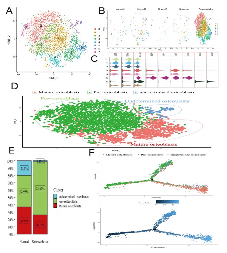
Osteoarthritis (OA) is the most common degenerative joint disease caused by osteoblastic lineage cells. However, a comprehensive molecular program for osteoblasts in human OA remains underdeveloped. The single-cell gene expression of osteoblasts and microRNA array data were from human. After processing the single-cell RNA sequencing (scRNA-seq) data, it was subjected to principal component analysis (PCA) and T-Stochastic neighbor embedding analysis (TSNE). Differential expression analysis was aimed to find marker genes. Gene-ontology (GO) enrichment, Kyoto encyclopedia of genes and genomes (KEGG) pathway enrichment analysis and Gene set enrichment analysis (GSEA) were applied to characterize the molecular function of osteoblasts with marker genes. Protein–protein interaction (PPI) networks and core module were established for marker genes by using the STRING database and Cytoscape software. All nodes in the core module were considered to be hub genes. Subsequently, we predicted the potential miRNA of hub genes through the miRWalk, miRDB and TargetScan database and experimentally verified the miRNA by GSE105027. Finally, miRNA-mRNA regulatory network was constructed using the Cytoscape software. We characterized the single-cell expression profiling of 4387 osteoblasts from normal and OA sample. The proportion of osteoblasts subpopulations changed dramatically in the OA, with 70.42% of the pre-osteoblasts. 117 marker genes were included and the results of GO analysis show that up-regulated marker genes enriched in collagen-containing extracellular matrix were highly expressed in the pre-osteoblasts cluster. Both KEGG and GSEA analyses results indicated that IL-17 and NOD-like receptor signaling pathways were enriched in down-regulated marker genes. We visualize the weight of marker genes and constructed the core module in PPI network. In potential mRNA-miRNA regulatory network, hsa-miR-449a and hsa-miR-218-5p may be involved in the development of OA. Our study found that alterations in osteoblasts state and cellular molecular function in the subchondral bone region may be involved in the pathogenesis of osteoarthritis.
Citation: Changxiang Huan, Jiaxin Gao. Insight into the potential pathogenesis of human osteoarthritis via single-cell RNA sequencing data on osteoblasts[J]. Mathematical Biosciences and Engineering, 2022, 19(6): 6344-6361. doi: 10.3934/mbe.2022297
Osteoarthritis (OA) is the most common degenerative joint disease caused by osteoblastic lineage cells. However, a comprehensive molecular program for osteoblasts in human OA remains underdeveloped. The single-cell gene expression of osteoblasts and microRNA array data were from human. After processing the single-cell RNA sequencing (scRNA-seq) data, it was subjected to principal component analysis (PCA) and T-Stochastic neighbor embedding analysis (TSNE). Differential expression analysis was aimed to find marker genes. Gene-ontology (GO) enrichment, Kyoto encyclopedia of genes and genomes (KEGG) pathway enrichment analysis and Gene set enrichment analysis (GSEA) were applied to characterize the molecular function of osteoblasts with marker genes. Protein–protein interaction (PPI) networks and core module were established for marker genes by using the STRING database and Cytoscape software. All nodes in the core module were considered to be hub genes. Subsequently, we predicted the potential miRNA of hub genes through the miRWalk, miRDB and TargetScan database and experimentally verified the miRNA by GSE105027. Finally, miRNA-mRNA regulatory network was constructed using the Cytoscape software. We characterized the single-cell expression profiling of 4387 osteoblasts from normal and OA sample. The proportion of osteoblasts subpopulations changed dramatically in the OA, with 70.42% of the pre-osteoblasts. 117 marker genes were included and the results of GO analysis show that up-regulated marker genes enriched in collagen-containing extracellular matrix were highly expressed in the pre-osteoblasts cluster. Both KEGG and GSEA analyses results indicated that IL-17 and NOD-like receptor signaling pathways were enriched in down-regulated marker genes. We visualize the weight of marker genes and constructed the core module in PPI network. In potential mRNA-miRNA regulatory network, hsa-miR-449a and hsa-miR-218-5p may be involved in the development of OA. Our study found that alterations in osteoblasts state and cellular molecular function in the subchondral bone region may be involved in the pathogenesis of osteoarthritis.

| [1] |
B. Abramoff, F. E. Caldera, Osteoarthritis: pathology, diagnosis, and treatment options, Med. Clin. North Am., 104 (2020), 293-311. https://doi.org/10.1016/j.mcna.2019.10.007 doi: 10.1016/j.mcna.2019.10.007

|
| [2] |
R. C. Lawrence, D. T. Felson, C. G. Helmick, L. M. Arnold, H. Choi, R. A. Deyo, et al., Estimates of the prevalence of arthritis and other rheumatic conditions in the United States: Part Ⅱ, Arthritis Rheum., 58 (2008), 26-35. https://doi.org/10.1002/art.23176 doi: 10.1002/art.23176
|
| [3] |
S. Glyn-Jones, A. J. Palmer, R. Agricola, A. J. Price, T. L. Vincent, H. Weinans, et al., Osteoarthritis, Lancet, 386 (2015), 376-387. https://doi.org/10.1016/s0140-6736(14)60802-3 doi: 10.1016/s0140-6736(14)60802-3
|
| [4] |
C. Buckland-Wright, Subchondral bone changes in hand and knee osteoarthritis detected by radiography, Osteoarthritis Cartilage, 12 (2004), S10-19. https://doi.org/10.1016/j.joca.2003.09.007 doi: 10.1016/j.joca.2003.09.007
|
| [5] |
E. Dall'Ara, C. Ohman, M. Baleani, M. Viceconti, Reduced tissue hardness of trabecular bone is associated with severe osteoarthritis, J. Biomech., 44 (2011), 1593-1598. https://doi.org/10.1016/j.jbiomech.2010.12.022 doi: 10.1016/j.jbiomech.2010.12.022
|
| [6] |
D. M. Findlay, G. J. Atkins, Osteoblast-chondrocyte interactions in osteoarthritis, Curr. Osteoporosis Rep., 12 (2014), 127-134. https://doi.org/10.1007/s11914-014-0192-5 doi: 10.1007/s11914-014-0192-5
|
| [7] |
I. Prasadam, S. Farnaghi, J. Q. Feng, W. Gu, S. Perry, R. Crawford, et al., Impact of extracellular matrix derived from osteoarthritis subchondral bone osteoblasts on osteocytes: role of integrinβ1 and focal adhesion kinase signaling cues, Arthritis Res. Ther., 15 (2013), R150. https://doi.org/10.1186/ar4333 doi: 10.1186/ar4333
|
| [8] |
S. K. Tat, J. P. Pelletier, N. Amiable, C. Boileau, D. Lajeunesse, N. Duval, et al., Activation of the receptor EphB4 by its specific ligand ephrin B2 in human osteoarthritic subchondral bone osteoblasts, Arthritis Rheum., 58 (2008), 3820-3830. https://doi.org/10.1002/art.24029 doi: 10.1002/art.24029
|
| [9] | S. K. Tat, J. P. Pelletier, D. Lajeunesse, H. Fahmi, M. Lavigne, J. Martel-Pelletier, The differential expression of osteoprotegerin (OPG) and receptor activator of nuclear factor kappaB ligand (RANKL) in human osteoarthritic subchondral bone osteoblasts is an indicator of the metabolic state of these disease cells, Clin. Exp. Rheumatol., 26 (2008), 295-304. |
| [10] |
I. Prasadam, R. Crawford, Y. Xiao, Aggravation of ADAMTS and matrix metalloproteinase production and role of ERK1/2 pathway in the interaction of osteoarthritic subchondral bone osteoblasts and articular cartilage chondrocytes-possible pathogenic role in osteoarthritis, J. Rheumatol., 39 (2012), 621-634. https://doi.org/10.3899/jrheum.110777 doi: 10.3899/jrheum.110777
|
| [11] |
S. J. Rice, K. Cheung, L. N. Reynard, J. Loughlin, Discovery and analysis of methylation quantitative trait loci (mQTLs) mapping to novel osteoarthritis genetic risk signals, Osteoarthritis Cartilage, 27 (2019), 1545-1556. https://doi.org/10.1016/j.joca.2019.05.017 doi: 10.1016/j.joca.2019.05.017
|
| [12] |
S. J. Rice, F. Beier, D. A. Young, J. Loughlin, Interplay between genetics and epigenetics in osteoarthritis, Nat. Rev. Rheumatol., 16 (2020), 268-281. https://doi.org/10.1038/s41584-020-0407-3 doi: 10.1038/s41584-020-0407-3
|
| [13] |
P. Y. Huang, J. G. Wu, J. Gu, T. Q. Zhang, L. F. Li, S. Q. Wang, et al., Bioinformatics analysis of miRNA and mRNA expression profiles to reveal the key miRNAs and genes in osteoarthritis, J. Orthop. Surg. Res., 16 (2021), 63. https://doi.org/10.1186/s13018-021-02201-2 doi: 10.1186/s13018-021-02201-2
|
| [14] |
J. Luo, X. Luo, Z. Duan, W. Bai, X. Che, Z. Shan, et al., Comprehensive analysis of lncRNA and mRNA based on expression microarray profiling reveals different characteristics of osteoarthritis between Tibetan and Han patients, J. Orthop. Surg. Res., 16 (2021), 133. https://doi.org/10.1186/s13018-021-02213-y doi: 10.1186/s13018-021-02213-y
|
| [15] |
J. Xu, Y. Zeng, H. Si, Y. Liu, M. Li, J. Zeng, et al., Integrating transcriptome-wide association study and mRNA expression profile identified candidate genes related to hand osteoarthritis, Arthritis Res. Ther., 23 (2021), 81. https://doi.org/10.1186/s13075-021-02458-2 doi: 10.1186/s13075-021-02458-2
|
| [16] |
C. Li, J. Luo, X. Xu, Z. Zhou, S. Ying, X. Liao, et al., Single cell sequencing revealed the underlying pathogenesis of the development of osteoarthritis, Gene, 757 (2020), 144939. https://doi.org/10.1016/j.gene.2020.144939 doi: 10.1016/j.gene.2020.144939
|
| [17] |
Z. Wu, L. Shou, J, Wang, X. Xu, Identification of the key gene and pathways associated with osteoarthritis via single-cell RNA sequencing on synovial fibroblasts, Medicine (Baltimore), 99 (2020), e21707. https://doi.org/10.1097/md.0000000000021707 doi: 10.1097/md.0000000000021707
|
| [18] |
Q. Sun, S. Liu, J. Feng, Y. Kang, Y. Zhou, S. Guo, Current status of microRNAs that target the wnt signaling pathway in regulation of osteogenesis and bone metabolism: A review, Med. Sci. Monit., 27 (2021), e929510. https://doi.org/10.12659/msm.929510 doi: 10.12659/msm.929510
|
| [19] | T. E. Swingler, L. Niu, P. Smith, P. Paddy, L. Le, M. J. Barter, et al., The function of microRNAs in cartilage and osteoarthritis, Clin. Exp. Rheumatol., 37 (2019), 40-47. |
| [20] |
H. Tao, L. Cheng, R. Yang, Downregulation of miR-34a promotes proliferation and inhibits apoptosis of rat osteoarthritic cartilage cells by activating PI3K/Akt pathway, Clin. Interv. Aging, 15 (2020), 373-385. https://doi.org/10.2147/cia.S241855 doi: 10.2147/cia.S241855
|
| [21] |
X. Qiu, Y. Liu, H. Shen, Z. Wang, Y. Gong, J. Yang, et al., Single-cell RNA sequencing of human femoral head in vivo, Aging (Albany NY), 13 (2021), 15595-15619. https://doi.org/10.18632/aging.203124 doi: 10.18632/aging.203124
|
| [22] |
Y. Gong, J. Yang, X. Li, C. Zhou, Y. Chen, Z. Wang, et al., A systematic dissection of human primary osteoblasts in vivo at single-cell resolution, Aging (Albany NY), 13 (2021), 20629-20650. https://doi.org/10.18632/aging.203452 doi: 10.18632/aging.203452
|
| [23] |
A. Butler, P. Hoffman, P. Smibert, E. Papalexi, R. Satija, Integrating single-cell transcriptomic data across different conditions, technologies, and species, Nat. Biotechnol., 36 (2018), 411-420. https://doi.org/10.1038/nbt.4096 doi: 10.1038/nbt.4096
|
| [24] |
S. Lall, D. Sinha, S. Bandyopadhyay, D. Sengupta, Structure-aware principal component analysis for single-cell RNA-seq data, J. Comput. Biol., (2018). https://doi.org/10.1089/cmb.2018.0027 doi: 10.1089/cmb.2018.0027
|
| [25] |
F. Pont, M. Tosolini, J. J. Fournié, Single-Cell Signature Explorer for comprehensive visualization of single cell signatures across scRNA-seq datasets, Nucleic Acids Res., 47 (2019), e133. https://doi.org/10.1093/nar/gkz601 doi: 10.1093/nar/gkz601
|
| [26] |
A. N. Tikhonova, I. Dolgalev, H. Hu, K. K. Sivaraj, E. Hoxha, Á. Cuesta-Domínguez, et al., The bone marrow microenvironment at single-cell resolution, Nature, 569 (2019), 222-228. https://doi.org/10.1038/s41586-019-1104-8 doi: 10.1038/s41586-019-1104-8
|
| [27] |
Y. Matsushita, M. Nagata, K. M. Kozloff, J. D. Welch, K. Mizuhashi, N. Tokavanich, et al., A Wnt-mediated transformation of the bone marrow stromal cell identity orchestrates skeletal regeneration, Nat. Commun., 11 (2020), 332. https://doi.org/10.1038/s41467-019-14029-w doi: 10.1038/s41467-019-14029-w
|
| [28] |
X. Qiu, Q. Mao, Y. Tang, L. Wang, R. Chawla, H. A. Pliner, et al., Reversed graph embedding resolves complex single-cell trajectories, Nat. Methods, 14 (2017), 979-982. https://doi.org/10.1038/nmeth.4402 doi: 10.1038/nmeth.4402
|
| [29] |
G. Yu, L. G. Wang, Y. Han, Q. Y. He, clusterProfiler: an R package for comparing biological themes among gene clusters, Omics, 16 (2012), 284-287. https://doi.org/10.1089/omi.2011.0118 doi: 10.1089/omi.2011.0118
|
| [30] |
P. Shannon, A. Markiel, O. Ozier, N. S. Baliga, J. T. Wang, D. Ramage, et al., Cytoscape: a software environment for integrated models of biomolecular interaction networks, Genome Res., 13 (2003), 2498-2504. https://doi.org/10.1101/gr.1239303 doi: 10.1101/gr.1239303
|
| [31] |
M. E. Ritchie, B. Phipson, D. Wu, Y. Hu, C. W. Law, W. Shi, et al., limma powers differential expression analyses for RNA-sequencing and microarray studies, Nucleic Acids Res., 43 (2015), e47. https://doi.org/10.1093/nar/gkv007 doi: 10.1093/nar/gkv007
|
| [32] |
N. Maruotti, A. Corrado, F. P. Cantatore, Osteoblast role in osteoarthritis pathogenesis, J. Cell Physiol., 232 (2017), 2957-2963. https://doi.org/10.1002/jcp.25969 doi: 10.1002/jcp.25969
|
| [33] |
I. Titorencu, V. Pruna, V. V. Jinga, M. Simionescu, Osteoblast ontogeny and implications for bone pathology: an overview, Cell Tissue Res., 355 (2014), 23-33. https://doi.org/10.1007/s00441-013-1750-3 doi: 10.1007/s00441-013-1750-3
|
| [34] |
A. D. Theocharis, D. Manou, N. K. Karamanos, The extracellular matrix as a multitasking player in disease, Febs J., 286 (2019), 2830-2869. https://doi.org/10.1111/febs.14818 doi: 10.1111/febs.14818
|
| [35] |
H. Z. Li, H. D. Lu, Transcriptome analyses identify key genes and potential mechanisms in a rat model of osteoarthritis, J. Orthop. Surg. Res., 13 (2018), 319. https://doi.org/10.1186/s13018-018-1019-3 doi: 10.1186/s13018-018-1019-3
|
| [36] |
Y. Shi, X. Hu, J. Cheng, X. Zhang, F. Zhao, W. Shi, et al., A small molecule promotes cartilage extracellular matrix generation and inhibits osteoarthritis development, Nat. Commun., 10 (2019), 1914. https://doi.org/10.1038/s41467-019-09839-x doi: 10.1038/s41467-019-09839-x
|
| [37] |
J. Y. Li, M. Yu, A. M. Tyagi, C. Vaccaro, E. Hsu, J. Adams, et al., IL-17 receptor signaling in osteoblasts/osteocytes mediates PTH-induced bone loss and enhances osteocytic RANKL production, J. Bone Miner Res., 34 (2019), 349-360. https://doi.org/10.1002/jbmr.3600 doi: 10.1002/jbmr.3600
|
| [38] |
Z. Wang, J. Tan, L. Lei, W. Sun, Y. Wu, P. Ding, et al., The positive effects of secreting cytokines IL-17 and IFN-γ on the early-stage differentiation and negative effects on the calcification of primary osteoblasts in vitro, Int. Immunopharmacol., 57 (2018), 1-10. https://doi.org/10.1016/j.intimp.2018.02.002 doi: 10.1016/j.intimp.2018.02.002
|
| [39] |
H. Kitaura, A. Marahleh, F. Ohori, T. Noguchi, W. R. Shen, J. Qi, et al., Osteocyte-related cytokines regulate osteoclast formation and bone resorption, Int. J. Mol. Sci., 21 (2020). https://doi.org/10.3390/ijms21145169 doi: 10.3390/ijms21145169
|
| [40] |
N. Udagawa, M. Koide, M. Nakamura, Y. Nakamichi, T. Yamashita, S. Uehara, et al., Osteoclast differentiation by RANKL and OPG signaling pathways, J. Bone Miner Metab., 39 (2021), 19-26. https://doi.org/10.1007/s00774-020-01162-6 doi: 10.1007/s00774-020-01162-6
|
| [41] |
M. Croes, F. C. Öner, D. van Neerven, E. Sabir, M. C. Kruyt, T. J. Blokhuis, et al., Proinflammatory T cells and IL-17 stimulate osteoblast differentiation, Bone, 84 (2016), 262-270. https://doi.org/10.1016/j.bone.2016.01.010 doi: 10.1016/j.bone.2016.01.010
|
| [42] |
S. Shen, Y. Wu, J. Chen, Z. Xie, K. Huang, G. Wang, et al., CircSERPINE2 protects against osteoarthritis by targeting miR-1271 and ETS-related gene, Ann. Rheum. Dis., 78 (2019), 826-836. https://doi.org/10.1136/annrheumdis-2018-214786 doi: 10.1136/annrheumdis-2018-214786
|
| [43] |
Y. Chao, L. Zhang, X. Zhang, C. Ma, Z. Chen, Expression of MiR-140 and MiR-199 in synovia and its correlation with the progression of knee osteoarthritis, Med. Sci. Monit., 26 (2020), e918174. https://doi.org/10.12659/msm.918174 doi: 10.12659/msm.918174
|
| [44] |
B. Zhang, M. Sun, J. Wang, C. Ma, T. Hao, G. Liu, et al., MiR-671 ameliorates the progression of osteoarthritis in vitro and in vivo, Pathol. Res. Pract., 215 (2019), 152423. https://doi.org/10.1016/j.prp.2019.04.015 doi: 10.1016/j.prp.2019.04.015
|
| [45] |
Z. Rasheed, H. A. Al-Shobaili, N. Rasheed, A. A. Al Salloom, O. Al-Shaya, A. Mahmood, et al., Integrated study of globally expressed microRNAs in IL-1β-stimulated human osteoarthritis chondrocytes and osteoarthritis relevant genes: A microarray and bioinformatics analysis, Nucleosides Nucleotides Nucleic Acids, 35 (2016), 335-355. https://doi.org/10.1080/15257770.2016.1163380 doi: 10.1080/15257770.2016.1163380
|
| [46] |
A. Soyocak, H. Kurt, M. Ozgen, D. Turgut Cosan, E. Colak, H. V. Gunes, miRNA-146a, miRNA-155 and JNK expression levels in peripheral blood mononuclear cells according to grade of knee osteoarthritis, Gene, 627 (2017), 207-211. https://doi.org/10.1016/j.gene.2017.06.027 doi: 10.1016/j.gene.2017.06.027
|
| [47] | G. Wang, Y. Zhang, X. Zhao, C. Meng, L. Ma, Y. Kong, MicroRNA-411 inhibited matrix metalloproteinase 13 expression in human chondrocytes, Am. J. Transl. Res., 7 (2015), 2000-2006. |
| [48] |
E. Nemoto, T. Honda, S. Kanaya, H. Takada, H. Shimauchi, Expression of functional Toll-like receptors and nucleotide-binding oligomerization domain proteins in murine cementoblasts and their upregulation during cell differentiation, J. Periodontal. Res., 43 (2008), 585-593. https://doi.org/10.1111/j.1600-0765.2008.01096.x doi: 10.1111/j.1600-0765.2008.01096.x
|
 mbe-19-06-297-supplementary.pdf mbe-19-06-297-supplementary.pdf |
 |


Figures(6)

Changxiang Huan, Jiaxin Gao. Insight into the potential pathogenesis of human osteoarthritis via single-cell RNA sequencing data on osteoblasts[J]. Mathematical Biosciences and Engineering, 2022, 19(6): 6344-6361. doi: 10.3934/mbe.2022297


 DownLoad: