Stability of stochastic nonlinear systems under aperiodically intermittent state quantization and event-triggered mechanism

Biwen Li; Guangyu Wang; Biwen Li; Guangyu Wang

doi:10.3934/math.2025459

AIMS Mathematics

2025, Volume 10, Issue 4: 10062-10092. doi: 10.3934/math.2025459

Previous Article Next Article

Research article

Stability of stochastic nonlinear systems under aperiodically intermittent state quantization and event-triggered mechanism

Biwen Li ,
Guangyu Wang ^,

School of Mathematics and Statistics, Hubei Normal University, Huangshi 435002, China

Received: 15 February 2025 Revised: 24 March 2025 Accepted: 10 April 2025 Published: 28 April 2025
MSC : 93C10, 93D40

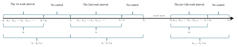
This work investigates the event-triggered control (ETC) problem for stochastic nonlinear systems with intermittent control (IC) and state quantization. ETC, state quantization, and aperiodically intermittent control (APIC) are incorporated into the control scheme to reduce the computational cost and communication load. Within the APIC framework, two control strategies are considered to examine their interactions: state quantization before event triggering (QbE) and state quantization after event triggering (QaE). Additionally, the Zeno phenomenon is avoided in the design of two static event-triggered mechanisms (ETMs). The known input-to-state stability (ISS) control law is supported by the system. Finite-time stability (FTS) and finite-time contraction stability (FTCS) are implemented. Each strategy guarantees the system's stability, and the appropriate scheme can be chosen by adjusting the length of the control interval. The effectiveness of the proposed ETC method is demonstrated through two numerical simulations.
- stochastic nonlinear systems,
- state quantization,
- event-triggered mechanism,
- finite-time stability,
- aperiodically intermittent control
Citation: Biwen Li, Guangyu Wang. Stability of stochastic nonlinear systems under aperiodically intermittent state quantization and event-triggered mechanism[J]. AIMS Mathematics, 2025, 10(4): 10062-10092. doi: 10.3934/math.2025459

Related Papers:

Abstract

This work investigates the event-triggered control (ETC) problem for stochastic nonlinear systems with intermittent control (IC) and state quantization. ETC, state quantization, and aperiodically intermittent control (APIC) are incorporated into the control scheme to reduce the computational cost and communication load. Within the APIC framework, two control strategies are considered to examine their interactions: state quantization before event triggering (QbE) and state quantization after event triggering (QaE). Additionally, the Zeno phenomenon is avoided in the design of two static event-triggered mechanisms (ETMs). The known input-to-state stability (ISS) control law is supported by the system. Finite-time stability (FTS) and finite-time contraction stability (FTCS) are implemented. Each strategy guarantees the system's stability, and the appropriate scheme can be chosen by adjusting the length of the control interval. The effectiveness of the proposed ETC method is demonstrated through two numerical simulations.

References

[1]	Z. G. Yan, F. X. Su, Z. W. Gao, Mean‐square strong stability and stabilization of discrete‐time stochastic systems with multiplicative noises, Int. J. Robust Nonlinear Control, 32 (2022), 6767–6784. https://doi.org/10.1002/rnc.6161 doi: 10.1002/rnc.6161
[2]	L. Arnold, Stochastic differential equations: Theory and applications, Wiley, 1974.
[3]	X. R. Mao, Stochastic differential equations and applications, Elsevier, 2007.
[4]	G. Ling, X. Z. Liu, Z. H. Guan, M. F. Ge, Y. H. Tong, Input-to-state stability for switched stochastic nonlinear systems with mode-dependent random impulses, Inform. Sciences, 596 (2022), 588–607. https://doi.org/10.1016/j.ins.2022.03.034 doi: 10.1016/j.ins.2022.03.034
[5]	X. R. Mao, Stabilization of continuous-time hybrid stochastic differential equations by discrete-time feedback control, Automatica, 49 (2013), 3677–3681. https://doi.org/10.1016/j.automatica.2013.09.005 doi: 10.1016/j.automatica.2013.09.005
[6]	W. C. Zou, P. Shi, Z. R. Xiang, Y. Shi, Consensus tracking control of switched stochastic nonlinear multiagent systems via event-triggered strategy, IEEE Trans. Neural Netw. Learn. Syst., 31 (2020), 1036–1045. https://doi.org/10.1109/TNNLS.2019.2917137 doi: 10.1109/TNNLS.2019.2917137
[7]	Q. X. Zhu, Stabilization of stochastic nonlinear delay systems with exogenous disturbances and the event-triggered feedback control, IEEE Trans. Autom. Control, 64 (2019), 3764–3771. https://doi.org/10.1109/TAC.2018.2882067 doi: 10.1109/TAC.2018.2882067
[8]	Y. F. Gao, X. M. Sun, C. Y. Wen, W. Wang, Event-triggered control for stochastic nonlinear systems, Automatica, 95 (2018), 534–538. https://doi.org/10.1016/j.automatica.2018.05.021 doi: 10.1016/j.automatica.2018.05.021
[9]	S. X. Luo, F. Q. Deng, On event-triggered control of nonlinear stochastic systems, IEEE Trans. Autom. Control, 65 (2020), 369–375. https://doi.org/10.1109/TAC.2019.2916285 doi: 10.1109/TAC.2019.2916285
[10]	X. T. Yang, Q. X. Zhu, Stabilization of stochastic nonlinear systems via double-event-triggering mechanisms and switching controls, Chaos Soliton Fract., 183 (2024), 114880. https://doi.org/10.1016/j.chaos.2024.114880 doi: 10.1016/j.chaos.2024.114880
[11]	T. F. Liu, P. P. Zhang, Z. P. Jiang, Event-triggered input-to-state stabilization of nonlinear systems subject to disturbances and dynamic uncertainties, Automatica, 108 (2019), 108488. https://doi.org/10.1016/j.automatica.2019.07.001 doi: 10.1016/j.automatica.2019.07.001
[12]	M. Liu, H. J. Jiang, C. Hu, Finite-time synchronization of delayed dynamical networks via aperiodically intermittent control, J. Franklin Inst., 354 (2017), 5374–5397. https://doi.org/10.1016/j.jfranklin.2017.05.030 doi: 10.1016/j.jfranklin.2017.05.030
[13]	D. S. Xu, L. L. Li, C. K. Ahn, Y. B. Wu, H. Su, Intermittent event-triggered control for input-to-state stability of stochastic systems, Int. J. Robust Nonlinear Control, 34 (2024), 8495–8516. https://doi.org/10.1002/rnc.7417 doi: 10.1002/rnc.7417
[14]	X. D. Liu, F. Q. Deng, W. Wei, F. Z. Wan, P. L. Yu, Periodically intermittent control for stochastic nonlinear delay systems with dynamic event-triggered mechanism, Int. J. Robust Nonlinear Control, 33 (2023), 9665–9683. https://doi.org/10.1002/rnc.6867 doi: 10.1002/rnc.6867
[15]	T. R. Chen, J. C. Chen, Input-to-state stability of stochastic complex networks based on aperiodically intermittent sampled control, Neurocomputing, 570 (2024), 127100. https://doi.org/10.1016/j.neucom.2023.127100 doi: 10.1016/j.neucom.2023.127100
[16]	Y. Y. Sun, F. Q. Deng, P. L. Yu, Y. J. Huang, Aperiodically intermittent control of switched stochastic nonlinear systems based on discrete-time observation, IEEE Trans. Circuits Syst. II, 71 (2024), 345–349. https://doi.org/10.1109/TCSII.2023.3302949 doi: 10.1109/TCSII.2023.3302949
[17]	G. J. Shen, R. D. Xiao, X. W. Yin, J. H. Zhang, Stabilization for hybrid stochastic systems by aperiodically intermittent control, Nonlinear Anal-Hybri., 39 (2021), 100990. https://doi.org/10.1016/j.nahs.2020.100990 doi: 10.1016/j.nahs.2020.100990
[18]	Y. Guo, M. Y. Duan, P. F. Wang, Input-to-state stabilization of semilinear systems via aperiodically intermittent event-triggered control, IEEE Trans. Control Netw. Syst., 9 (2022), 731–741. https://doi.org/10.1109/TCNS.2022.3165511 doi: 10.1109/TCNS.2022.3165511
[19]	Z. Y. Yu, S. Z. Yu, H. J. Jiang, Finite/fixed-time event-triggered aperiodic intermittent control for nonlinear systems, Chaos Soliton Fract., 173 (2023), 113735. https://doi.org/10.1016/j.chaos.2023.113735 doi: 10.1016/j.chaos.2023.113735
[20]	Y. N. Wang, C. D. Li, H. J. Wu, H. Deng, Stabilization of nonlinear delayed systems subject to impulsive disturbance via aperiodic intermittent control, J. Franklin Inst., 361 (2024), 106675. https://doi.org/10.1016/j.jfranklin.2024.106675 doi: 10.1016/j.jfranklin.2024.106675
[21]	G. L. Wu, X. T. Wu, J. D. Cao, W. B. Zhang, Event-triggered aperiodic intermittent control for linear time-varying systems, ISA Trans., 144 (2024), 96–104. https://doi.org/10.1016/j.isatra.2023.11.005 doi: 10.1016/j.isatra.2023.11.005
[22]	M. Y. Fu, L. H. Xie, The sector bound approach to quantized feedback control, IEEE Trans. Autom. Control, 50 (2005), 1698–1711. https://doi.org/10.1109/TAC.2005.858689 doi: 10.1109/TAC.2005.858689
[23]	T. F. Liu, Z. P. Jiang, D. J. Hill, A sector bound approach to feedback control of nonlinear systems with state quantization, Automatica, 48 (2012), 145–152. https://doi.org/10.1016/j.automatica.2011.09.041 doi: 10.1016/j.automatica.2011.09.041
[24]	T. F. Liu, Z. P. Jiang, Quantized nonlinear control—a survey, Acta Autom. Sin., 39 (2013), 1820–1830. https://doi.org/10.1016/S1874-1029(13)60079-8 doi: 10.1016/S1874-1029(13)60079-8
[25]	T. F. Liu, Z. P. Jiang, Event-triggered control of nonlinear systems with state quantization, IEEE Trans. Autom. Control, 64 (2018), 797–803. https://doi.org/10.1109/TAC.2018.2837129 doi: 10.1109/TAC.2018.2837129
[26]	Y. Y. Sun, F. Q. Deng, P. L. Yu, Event-triggered control of It$\hat{\mathbf{o}}$ stochastic nonlinear delayed systems with state quantization, Int. J. Robust Nonlinear Control, 34 (2024), 3167–3188. https://doi.org/10.1002/rnc.7130 doi: 10.1002/rnc.7130
[27]	X. D. Li, X. Y. Yang, S. J. Song, Lyapunov conditions for finite-time stability of time-varying time-delay systems, Automatica, 103 (2019), 135–140. https://doi.org/10.1016/j.automatica.2019.01.031 doi: 10.1016/j.automatica.2019.01.031
[28]	B. Zhou, Finite-time stabilization of linear systems by bounded linear time-varying feedback, Automatica, 113 (2020), 108760. https://doi.org/10.1016/j.automatica.2019.108760 doi: 10.1016/j.automatica.2019.108760
[29]	M. Liu, H. J. Jiang, C. Hu, Finite-time synchronization of delayed dynamical networks via aperiodically intermittent control, J. Franklin Inst., 354 (2017), 5374–5397. https://doi.org/10.1016/j.jfranklin.2017.05.030 doi: 10.1016/j.jfranklin.2017.05.030
[30]	X. Y. Yang, X. D. Li, Finite-time stability of nonlinear impulsive systems with applications to neural networks, IEEE Trans. Neural Netw. Learn. Syst., 34 (2021), 243–251. https://doi.org/10.1109/TNNLS.2021.3093418 doi: 10.1109/TNNLS.2021.3093418
[31]	T. X. Zhang, X. D. Li, J. D. Cao, Finite-time stability of impulsive switched systems, IEEE Trans. Autom. Control, 68 (2022), 5592–5599. https://doi.org/10.1109/TAC.2022.3219294 doi: 10.1109/TAC.2022.3219294
[32]	L. Y. You, X. Y. Yang, S. C. Wu, X. D. Li, Finite-time stabilization for uncertain nonlinear systems with impulsive disturbance via aperiodic intermittent control, Appl. Math Comput., 443 (2023), 127782. https://doi.org/10.1016/j.amc.2022.127782 doi: 10.1016/j.amc.2022.127782
[33]	L. Y. You, S. C. Wu, X. D. Li, Finite-time stabilization of nonlinear systems via hybrid control and application to state estimation of complex networks, IEEE Trans. Autom. Sci. Eng., 22 (2025), 4154–4167. https://doi.org/10.1109/TASE.2024.3408105 doi: 10.1109/TASE.2024.3408105
[34]	T. Xu, J. E. Zhang, Intermittent control for stabilization of uncertain nonlinear systems via event-triggered mechanism, AIMS Mathematics, 9 (2024), 28487–28507. https://doi.org/10.3934/math.20241382 doi: 10.3934/math.20241382
[35]	L. Mchiri, A. B. Makhlouf, D. Baleanu, M. Rhaima, Finite-time stability of linear stochastic fractional-order systems with time delay, Adv. Differ. Equ., 2021 (2021), 345. https://doi.org/10.1186/s13662-021-03500-y doi: 10.1186/s13662-021-03500-y
[36]	J. Ge, L. Xie, S. Fang, K. Zhang, Lyapunov conditions for finite-time stability of stochastic functional systems, Int. J. Control Autom. Syst., 22 (2024), 106–115. https://doi.org/10.1007/s12555-022-0516-7 doi: 10.1007/s12555-022-0516-7
[37]	J. L. Yin, S. Y. Khoo, Z. H. Man, X. H. Yu, Finite-time stability and instability of stochastic nonlinear systems, Automatica, 47 (2011), 2671–2677. https://doi.org/10.1016/j.automatica.2011.08.050 doi: 10.1016/j.automatica.2011.08.050
[38]	J. Y. Liu, Q. X. Zhu, Finite time stability of nonlinear impulsive stochastic system and its application to neural networks, Commun. Nonlinear Sci. Numer. Simul., 139 (2024), 108298. https://doi.org/10.1016/j.cnsns.2024.108298 doi: 10.1016/j.cnsns.2024.108298
[39]	Y. Zhou, A. Polyakov, G. Zheng, Finite/fixed-time stabilization of linear systems with state quantization, IEEE Trans. Autom. Control, 70 (2025), 1921–1928. https://doi.org/10.1109/TAC.2024.3473619 doi: 10.1109/TAC.2024.3473619

Reader Comments

Your name:*

Email:*
© 2025 the Author(s), licensee AIMS Press. This is an open access article distributed under the terms of the Creative Commons Attribution License (http://creativecommons.org/licenses/by/4.0)