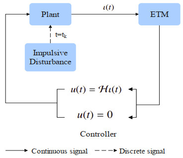
This paper studies the finite-time stabilization (FTS) and finite-time contraction stabilization (FTCS) of parameter-uncertain systems subjected to impulsive disturbances by using an event-triggered aperiodic intermittent control (EAPIC) method, which combines aperiodic intermittent control with event-triggered control. By employing the Lyapunov method and linear matrix inequality techniques, sufficient conditions for FTS and FTCS are derived. Additionally, within the finite-time control framework, relationships among impulsive disturbance, intermittent control parameters, and event-triggered mechanism (ETM) thresholds are established under EAPIC to ensure FTS and FTCS. The sequence of impulsive moments is determined by a predetermined ETM, and Zeno phenomena are also excluded. Finally, the effectiveness of the EAPIC approach is demonstrated through two numerical examples.
Citation: Tian Xu, Jin-E Zhang. Intermittent control for stabilization of uncertain nonlinear systems via event-triggered mechanism[J]. AIMS Mathematics, 2024, 9(10): 28487-28507. doi: 10.3934/math.20241382
This paper studies the finite-time stabilization (FTS) and finite-time contraction stabilization (FTCS) of parameter-uncertain systems subjected to impulsive disturbances by using an event-triggered aperiodic intermittent control (EAPIC) method, which combines aperiodic intermittent control with event-triggered control. By employing the Lyapunov method and linear matrix inequality techniques, sufficient conditions for FTS and FTCS are derived. Additionally, within the finite-time control framework, relationships among impulsive disturbance, intermittent control parameters, and event-triggered mechanism (ETM) thresholds are established under EAPIC to ensure FTS and FTCS. The sequence of impulsive moments is determined by a predetermined ETM, and Zeno phenomena are also excluded. Finally, the effectiveness of the EAPIC approach is demonstrated through two numerical examples.

| [1] |
K. T. Chang, Investigation of electrical transient behavior of an ultrasonic transducer under impulsive mechanical excitation, Sensors Actuat. A: Phys., 133 (2007), 407–414. https://doi.org/10.1016/j.sna.2006.04.017 doi: 10.1016/j.sna.2006.04.017

|
| [2] | A. Pentari, G. Tzagkarakis, K. Marias, P. Tsakalides, Graph-based denoising of EEG signals in impulsive environments, 2020 28th European Signal Processing Conference (EUSIPCO), IEEE, 2021, 1095–1099. https://doi.org/10.23919/Eusipco47968.2020.9287329 |
| [3] |
P. S. Rivadeneira, C. H. Moog, Observability criteria for impulsive control systems with applications to biomedical engineering processes, Automatica, 55 (2015), 125–131. https://doi.org/10.1016/j.automatica.2015.02.042 doi: 10.1016/j.automatica.2015.02.042
|
| [4] |
X. Y. Chen, Y. Liu, B. X. Jiang, J. Q. Lu, Exponential stability of nonlinear switched systems with hybrid delayed impulses, Int. J. Robust Nonlinear Control, 33 (2023), 2971–2985. https://doi.org/10.1002/rnc.6547 doi: 10.1002/rnc.6547
|
| [5] |
S. C. Wu, X. D. Li, Finite-time stability of nonlinear systems with delayed impulses, IEEE Trans. Syst. Man Cybern.: Syst., 53 (2023), 7453–7460. https://doi.org/10.1109/TSMC.2023.3298071 doi: 10.1109/TSMC.2023.3298071
|
| [6] |
X. Y. Yang, X. D. Li, P. Y. Duan, Finite-time lag synchronization for uncertain complex networks involving impulsive disturbances, Neural Comput. Appl., 34 (2022), 5097–5106. https://doi.org/10.1007/s00521-021-05987-8 doi: 10.1007/s00521-021-05987-8
|
| [7] |
Z. Y. Wang, X. Z. Liu, Exponential stability of impulsive complex-valued neural networks with time delay, Math. Comput. Simul., 156 (2019), 143–157. https://doi.org/10.1016/j.matcom.2018.07.006 doi: 10.1016/j.matcom.2018.07.006
|
| [8] |
W. Zhang, C. D. Li, T. W. Huang, J. Tan, Exponential stability of inertial BAM neural networks with time-varying delay via periodically intermittent control, Neural Comput. Appl., 26 (2015), 1781–1787. https://doi.org/10.1007/s00521-015-1838-7 doi: 10.1007/s00521-015-1838-7
|
| [9] |
Y. Liu, J. Liu, W. X. Li, Stabilization of highly nonlinear stochastic coupled systems via periodically intermittent control, IEEE Trans. Autom. Control, 66 (2020), 4799–4806. https://doi.org/10.1109/TAC.2020.3036035 doi: 10.1109/TAC.2020.3036035
|
| [10] |
W. H. Chen, J. C. Zhong, W. X. Zheng, Delay-independent stabilization of a class of time-delay systems via periodically intermittent control, Automatica, 71 (2016), 89–97. https://doi.org/10.1016/j.automatica.2016.04.031 doi: 10.1016/j.automatica.2016.04.031
|
| [11] |
Y. G. Wang, D. Li, Adaptive synchronization of chaotic systems with time-varying delay via aperiodically intermittent control, Soft Comput., 24 (2020), 12773–12780. https://doi.org/10.1007/s00500-020-05161-7 doi: 10.1007/s00500-020-05161-7
|
| [12] |
D. Liu, D. Ye, Exponential stabilization of delayed inertial memristive neural networks via aperiodically intermittent control strategy, IEEE Trans. Syst. Man Cybern.: Syst., 52 (2020), 448–458. https://doi.org/10.1109/TSMC.2020.3002960 doi: 10.1109/TSMC.2020.3002960
|
| [13] |
W. J. Sun, X. D. Li, Aperiodic intermittent control for exponential input-to-state stabilization of nonlinear impulsive systems, Nonlinear Anal., 50 (2023), 101404. https://doi.org/10.1016/j.nahs.2023.101404 doi: 10.1016/j.nahs.2023.101404
|
| [14] |
C. D. Li, G. Feng, X. F. Liao, Stabilization of nonlinear systems via periodically intermittent control, IEEE Trans. Circuits Syst. II, 54 (2007), 1019–1023. https://doi.org/10.1109/TCSII.2007.903205 doi: 10.1109/TCSII.2007.903205
|
| [15] |
B. Liu, M. Yang, T. Liu, D. J. Hill, Stabilization to exponential input-to-state stability via aperiodic intermittent control, IEEE Trans. Autom. Control, 66 (2020), 2913–2919. https://doi.org/10.1109/TAC.2020.3014637 doi: 10.1109/TAC.2020.3014637
|
| [16] |
X. R. Zhang, Q. Z. Wang, B. Z. Fu, Further stabilization criteria of continuous systems with aperiodic time-triggered intermittent control, Commun. Nonlinear Sci. Numer. Simul., 125 (2023), 107387. https://doi.org/10.1016/j.cnsns.2023.107387 doi: 10.1016/j.cnsns.2023.107387
|
| [17] |
T. F. Liu, Z. P. Jiang, Event-triggered control of nonlinear systems with state quantization, IEEE Trans. Autom. Control, 64 (2018), 797–803. https://doi.org/10.1109/TAC.2018.2837129 doi: 10.1109/TAC.2018.2837129
|
| [18] |
J. S. Huang, W. Wang, C. Y. Wen, G. Q. Li, Adaptive event-triggered control of nonlinear systems with controller and parameter estimator triggering, IEEE Trans. Autom. Control, 65 (2019), 318–324. https://doi.org/10.1109/TAC.2019.2912517 doi: 10.1109/TAC.2019.2912517
|
| [19] |
X. D. Li, D. X. Peng, J. D. Cao, Lyapunov stability for impulsive systems via event-triggered impulsive control, IEEE Trans. Autom. Control, 65 (2020), 4908–4913. https://doi.org/10.1109/TAC.2020.2964558 doi: 10.1109/TAC.2020.2964558
|
| [20] |
K. X. Zhang, B. Gharesifard, E. Braverman, Event-triggered control for nonlinear time-delay systems, IEEE Trans. Autom. Control, 67 (2021), 1031–1037. https://doi.org/10.1109/TAC.2021.3062577 doi: 10.1109/TAC.2021.3062577
|
| [21] |
B. Liu, T. Liu, P. Xiao, Dynamic event-triggered intermittent control for stabilization of delayed dynamical systems, Automatica, 149 (2023), 110847. https://doi.org/10.1016/j.automatica.2022.110847 doi: 10.1016/j.automatica.2022.110847
|
| [22] |
B. Liu, M. Yang, B. Xu, G. H. Zhang, Exponential stabilization of continuous-time dynamical systems via time and event triggered aperiodic intermittent control, Appl. Math. Comput., 398 (2021), 125713. https://doi.org/10.1016/j.amc.2020.125713 doi: 10.1016/j.amc.2020.125713
|
| [23] |
B. Zhou, Finite-time stability analysis and stabilization by bounded linear time-varying feedback, Automatica, 121 (2020), 109191. https://doi.org/10.1016/j.automatica.2020.109191 doi: 10.1016/j.automatica.2020.109191
|
| [24] |
X. Y. He, X. D. Li, S. J. Song, Finite-time input-to-state stability of nonlinear impulsive systems, Automatica, 135 (2022), 109994. https://doi.org/10.1016/j.automatica.2021.109994 doi: 10.1016/j.automatica.2021.109994
|
| [25] |
X. D. Li, X. Y. Yang, S. J. Song, Lyapunov conditions for finite-time stability of time-varying time-delay systems, Automatica, 103 (2019), 135–140. https://doi.org/10.1016/j.automatica.2019.01.031 doi: 10.1016/j.automatica.2019.01.031
|
| [26] |
Z. C. Wang, J. Sun, J. Chen, Y. Q. Bai, Finite-time stability of switched nonlinear time-delay systems, Int. J. Robust Nonlinear Control, 30 (2020), 2906–2919. https://doi.org/10.1002/rnc.4928 doi: 10.1002/rnc.4928
|
| [27] |
J. Ge, L. P. Xie, S. X. Fang, K. J. Zhang, Lyapunov conditions for finite-time stability of stochastic functional systems, Int. J. Control Autom. Syst., 22 (2024), 106–115. https://doi.org/10.1007/s12555-022-0516-7 doi: 10.1007/s12555-022-0516-7
|
| [28] |
X. Y. Zhang, C. D. Li, Finite-time stability of nonlinear systems with state-dependent delayed impulses, Nonlinear Dyn., 102 (2020), 197–210. https://doi.org/10.1007/s11071-020-05953-4 doi: 10.1007/s11071-020-05953-4
|
| [29] |
Y. N. Wang, C. D. Li, H. J. Wu, H. Deng, Stabilization of nonlinear delayed systems subject to impulsive disturbance via aperiodic intermittent control, J. Franklin Inst., 361 (2024), 106675. https://doi.org/10.1016/j.jfranklin.2024.106675 doi: 10.1016/j.jfranklin.2024.106675
|
| [30] |
X. Y. Zhang, C. D. Li, H. F. Li, Finite-time stabilization of nonlinear systems via impulsive control with state-dependent delay, J. Franklin Inst., 359 (2022), 1196–1214. https://doi.org/10.1016/j.jfranklin.2021.11.013 doi: 10.1016/j.jfranklin.2021.11.013
|
| [31] |
X. Y. Yang, X. D. Li, Finite-time stability of nonlinear impulsive systems with applications to neural networks, IEEE Trans. Neur. Net. Lear. Syst., 34 (2021), 243–251. https://doi.org/10.1109/TNNLS.2021.3093418 doi: 10.1109/TNNLS.2021.3093418
|
| [32] |
L. Y. You, X. Y. Yang, S. C. Wu, X. D. Li, Finite-time stabilization for uncertain nonlinear systems with impulsive disturbance via aperiodic intermittent control, Appl. Math. Comput., 443 (2023), 127782. https://doi.org/10.1016/j.amc.2022.127782 doi: 10.1016/j.amc.2022.127782
|
| [33] | F. Amato, R. Ambrosino, M. Ariola, C. Cosentino, G. D. Tommasi, Finite-time stability and control, Vol. 453, London: Springer, 2014. https://doi.org/10.1007/978-1-4471-5664-2 |
| [34] |
W. H. Chen, W. X. Zheng, Robust stability and $H_{\infty}$-control of uncertain impulsive systems with time-delay, Automatica, 45 (2009), 109–117. https://doi.org/10.1016/j.automatica.2008.05.020 doi: 10.1016/j.automatica.2008.05.020
|
| [35] |
E. N. Sanchez, J. P. Perez, Input-to-state stability (ISS) analysis for dynamic neural networks, IEEE Trans. Circuits Syst. I, 46 (1999), 1395–1398. https://doi.org/10.1109/81.802844 doi: 10.1109/81.802844
|
| [36] |
C. Xu, X. S. Yang, J. Q. Lu, J. W. Feng, F. E. Alsaadi, T. Hayat, Finite-time synchronization of networks via quantized intermittent pinning control, IEEE Trans. Cybern., 48 (2017), 3021–3027. https://doi.org/10.1109/TCYB.2017.2749248 doi: 10.1109/TCYB.2017.2749248
|
| [37] |
C. D. Li, X. F. Liao, T. W. Huang, Exponential stabilization of chaotic systems with delay by periodically intermittent control, Chaos, 17 (2007), 013103. https://doi.org/10.1063/1.2430394 doi: 10.1063/1.2430394
|


Figures(8)

Tian Xu, Jin-E Zhang. Intermittent control for stabilization of uncertain nonlinear systems via event-triggered mechanism[J]. AIMS Mathematics, 2024, 9(10): 28487-28507. doi: 10.3934/math.20241382


 DownLoad: