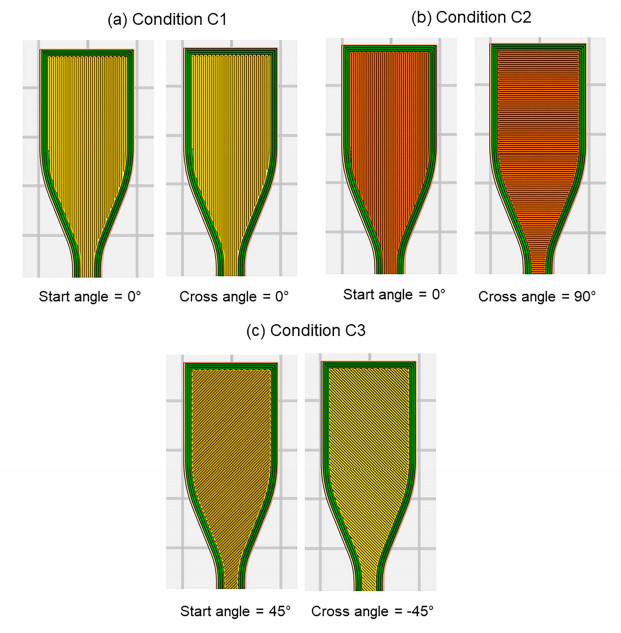
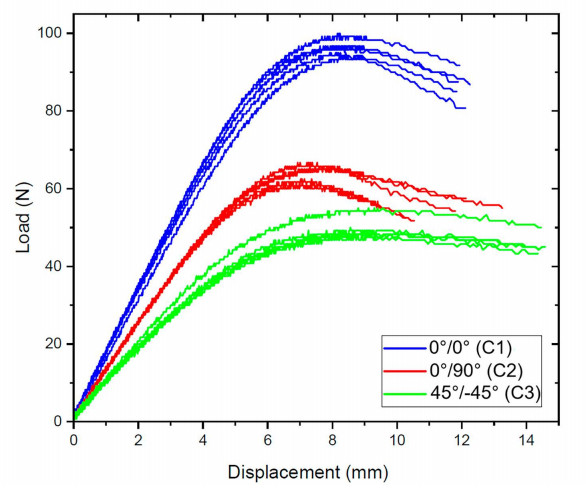
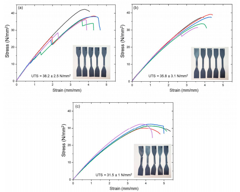
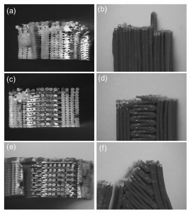
In fused deposition modeling (FDM) 3D printing, the properties and performance of the fabricated components are profoundly affected by the selected process parameters. Therefore, it is crucial to choose and optimize these parameters to improve the quality and mechanical characteristics of the final product. Given this, the present study explored the mechanical properties of 3D-printed components fabricated from polylactic acid (PLA)+ filament, specifically examining how different raster angles influence their flexural and tensile performance. Three raster angle conditions were investigated: parallel (0°/0°), grid (0°/90°), and crisscross (45°/−45°). The results demonstrate that the raster angle has a significant effect on the flexural and tensile strength of the printed specimens. The parallel raster (0°/0°) produced the highest flexural strength, attributed to the alignment of the fibers perpendicular to the applied load, which enhances the load capacity. Conversely, the crisscross (45°/−45°) orientation resulted in the lowest flexural strength but exhibited greater ductility, as evidenced by extensive plastic deformation. This increased ductility is attributed to the material's ability to absorb more energy before failure, resulting from favorable shear deformation dynamics. In tensile testing, the parallel raster (0°/0°) showed superior strength, while the grid and crisscross orientations followed with progressively lower values. The fracture behavior revealed that samples 3D printed with a 45°/−45° raster angle tend to fail along the raster orientation, primarily due to the development of shear stresses.
Citation: Juan Sebastián Ramírez-Prieto, Juan Sebastián Martínez-Yáñez, Andrés Giovanni González-Hernández. Effect of raster angle on the tensile and flexural strength of 3D printed PLA+ parts[J]. AIMS Materials Science, 2025, 12(2): 363-379. doi: 10.3934/matersci.2025019
In fused deposition modeling (FDM) 3D printing, the properties and performance of the fabricated components are profoundly affected by the selected process parameters. Therefore, it is crucial to choose and optimize these parameters to improve the quality and mechanical characteristics of the final product. Given this, the present study explored the mechanical properties of 3D-printed components fabricated from polylactic acid (PLA)+ filament, specifically examining how different raster angles influence their flexural and tensile performance. Three raster angle conditions were investigated: parallel (0°/0°), grid (0°/90°), and crisscross (45°/−45°). The results demonstrate that the raster angle has a significant effect on the flexural and tensile strength of the printed specimens. The parallel raster (0°/0°) produced the highest flexural strength, attributed to the alignment of the fibers perpendicular to the applied load, which enhances the load capacity. Conversely, the crisscross (45°/−45°) orientation resulted in the lowest flexural strength but exhibited greater ductility, as evidenced by extensive plastic deformation. This increased ductility is attributed to the material's ability to absorb more energy before failure, resulting from favorable shear deformation dynamics. In tensile testing, the parallel raster (0°/0°) showed superior strength, while the grid and crisscross orientations followed with progressively lower values. The fracture behavior revealed that samples 3D printed with a 45°/−45° raster angle tend to fail along the raster orientation, primarily due to the development of shear stresses.

| [1] |
Oteyaka MO, Cakir FH, Sofuoglu MA (2022) Effect of infill pattern and ratio on the flexural and vibration-damping characteristics of FDM printed PLA specimens. Mater Today Commun 33: 104912. https://doi.org/10.1016/j.mtcomm.2022.104912 doi: 10.1016/j.mtcomm.2022.104912

|
| [2] |
Rodríguez-Reyna SL, Mata C, Díaz-Aguilera JH, et al. (2023) Mechanical properties optimization for PLA, ABS and Nylon + CF manufactured by 3D FDM printing. Mater Today Commun 33: 104774. https://doi.org/10.1016/j.mtcomm.2022.104774 doi: 10.1016/j.mtcomm.2022.104774
|
| [3] |
Adibeig MR, Vakili-Tahami F, Saeimi-Sadigh MA (2023) Numerical and experimental investigation on creep response of 3D printed polylactic acid (PLA) samples. Part Ⅰ: The effect of building direction and unidirectional raster orientation. J Mech Behav Biomed Mater 145: 106025. https://doi.org/10.1016/j.jmbbm.2023.106025 doi: 10.1016/j.jmbbm.2023.106025
|
| [4] |
Medellin-Castillo HI, Zaragoza-Siqueiros J (2019) Design and manufacturing strategies for fused deposition modelling in additive manufacturing: A review. Chinese J Mech Eng 32: 1–16. https://doi.org/10.1186/s10033-019-0368-0 doi: 10.1186/s10033-019-0368-0
|
| [5] |
Güler Ö, Tatlı O (2021) Mechanical characterization of polylactic acid polymer 3D printed materials: The effects of infill geometry. Rev Metal 57: e202. https://doi.org/10.3989/revmetalm.202 doi: 10.3989/revmetalm.202
|
| [6] |
Hikmat M, Rostam S, Ahmed YM (2021) Investigation of tensile property-based Taguchi method of PLA parts fabricated by FDM 3D printing technology. Results Eng 11: 100264. https://doi.org/10.1016/j.rineng.2021.100264 doi: 10.1016/j.rineng.2021.100264
|
| [7] |
El Magri A, Vaudreuil S (2021) Optimizing the mechanical properties of 3D-printed PLA graphene composite using response surface methodology. Arch Mater Sci Eng 112: 13–22. https://doi.org/10.5604/01.3001.0015.5928 doi: 10.5604/01.3001.0015.5928
|
| [8] |
Dey A, Yodo N (2019) A systematic survey of FDM process parameter optimization and their influence on part characteristics. J Manuf Mater Process 3: 64–94. https://doi.org/10.3390/jmmp3030064 doi: 10.3390/jmmp3030064
|
| [9] |
Bhayana M, Singh J, Sharma A, et al. (2023) A review on optimized FDM 3D printed wood/PLA bio composite material characteristics. Mater Today Proc. https://doi.org/10.1016/j.matpr.2023.03.029 doi: 10.1016/j.matpr.2023.03.029
|
| [10] |
Patel R, Desai C, Kushwah S, et al. (2022) A review article on FDM process parameters in 3D printing for composite materials. Mater Today Proc 60: 2162–2166. https://doi.org/10.1016/j.matpr.2022.02.385 doi: 10.1016/j.matpr.2022.02.385
|
| [11] |
Wang G, Yang Y, Liu C, et al. (2023) 3D printed TPMS structural PLA/GO scaffold: Process parameter optimization, porous structure, mechanical and biological properties. J Mech Behav Biomed Mater 142: 105848. https://doi.org/10.1016/j.jmbbm.2023.105848 doi: 10.1016/j.jmbbm.2023.105848
|
| [12] |
Benamira M, Benhassine N, Ayad A, et al. (2023) Investigation of printing parameters effects on mechanical and failure properties of 3D printed PLA. Eng Fail Anal 148: 107218. https://doi.org/10.1016/j.engfailanal.2023.107218 doi: 10.1016/j.engfailanal.2023.107218
|
| [13] |
Lubombo C, Huneault MA (2018) Effect of infill patterns on the mechanical performance of lightweight 3D-printed cellular PLA parts. Mater Today Commun 17: 214–228. https://doi.org/10.1016/j.mtcomm.2018.09.017 doi: 10.1016/j.mtcomm.2018.09.017
|
| [14] |
Almansoori K, Pervaiz S (2023) Effect of layer height, print speed and cell geometry on mechanical properties of marble PLA based 3D printed parts. Smart Mater Manuf 1: 100023. https://doi.org/10.1016/j.smmf.2023.100023 doi: 10.1016/j.smmf.2023.100023
|
| [15] |
Karimi HR, Khedri E, Nazemzadeh N, et al. (2023) Effect of layer angle and ambient temperature on the mechanical and fracture characteristics of unidirectional 3D printed PLA material. Mater Today Commun 35: 106174. https://doi.org/10.1016/j.mtcomm.2023.106174 doi: 10.1016/j.mtcomm.2023.106174
|
| [16] |
Saravana Kumar M, Farooq MU, Ross NS, et al. (2023) Achieving effective interlayer bonding of PLA parts during the material extrusion process with enhanced mechanical properties. Sci Rep 13: 6800. https://doi.org/10.1038/s41598-023-33510-7 doi: 10.1038/s41598-023-33510-7
|
| [17] |
Camargo JC, Machado AR, Almeida EC, et al. (2019) Mechanical properties of PLA-graphene filament for FDM 3D printing. Int J Adv Manuf Technol 103: 2423–2443. https://doi.org/10.1007/s00170-019-03532-5 doi: 10.1007/s00170-019-03532-5
|
| [18] |
Karad AS, Sonawwanay PD, Naik M, et al. (2023) Experimental study of effect of infill density on tensile and flexural strength of 3D printed parts. J Eng Appl Sci 70: 104. https://doi.org/10.1186/s44147-023-00273-x doi: 10.1186/s44147-023-00273-x
|
| [19] |
Karad AS, Sonawwanay PD, Naik M, et al. (2023) Experimental tensile strength analysis of ABS material through FDM technique. Mater Today Proc 103: 506–512. https://doi.org/10.1016/j.matpr.2023.09.216 doi: 10.1016/j.matpr.2023.09.216
|
| [20] |
Khan SF, Zakaria H, Chong YL, et al. (2018) Effect of infill on tensile and flexural strength of 3D printed PLA parts. IOP Conf Ser Mater Sci Eng 429: 012101. https://doi.org/10.1088/1757-899X/429/1/012101 doi: 10.1088/1757-899X/429/1/012101
|
| [21] |
Tanveer MQ, Mishra G, Mishra S, et al. (2022) Effect of infill pattern and infill density on mechanical behaviour of FDM 3D printed parts—A current review. Mater Today Proc 62: 100–108. https://doi.org/10.1016/j.matpr.2022.02.310 doi: 10.1016/j.matpr.2022.02.310
|
| [22] | Letcher T, Waytashek M (2014) Material property testing of 3D-printed specimen in PLA on an entry-level 3D printer. ASME 2014 International Mechanical Engineering Congress and Exposition, Montreal, Quebec, Canada. https://doi.org/10.1115/IMECE2014-39379 |
| [23] |
Balasubramanian M, Saravanan R, Sathish T, et al. (2024) Investigating the influence of strain rate on tensile, flexural, and ILSS of fused deposition modeling printed PLA polymer. J Mater Eng Perform. https://doi.org/10.1007/s11665-024-10180-8 doi: 10.1007/s11665-024-10180-8
|
| [24] |
Gajjar T, Yang RC, Ye L, et al. (2025) Effects of key process parameters on tensile properties and interlayer bonding behavior of 3D printed PLA using fused filament fabrication. Prog Addit Manuf 10: 1261–1280. https://doi.org/10.1007/s40964-024-00704-y doi: 10.1007/s40964-024-00704-y
|
| [25] |
Hasan A, Fahad M, Khan MA (2024) Effect of print parameters on the tensile strength and built time of FDM-printed PLA parts. Int J Adv Manuf Technol 132: 3047–3065. https://doi.org/10.1007/s00170-024-13506-x doi: 10.1007/s00170-024-13506-x
|
| [26] |
Ambade V, Rajurkar S, Awari G, et al. (2025) Influence of FDM process parameters on tensile strength of parts printed by PLA material. Int J Interact Des Manuf 19: 573–584. https://doi.org/10.1007/s12008-023-01490-7 doi: 10.1007/s12008-023-01490-7
|
| [27] |
Gopi Mohan R, Santhosh K, Iyer RV, et al. (2021) Comparative analysis of mechanical properties of FDM printed parts based on raster angles. Mater Today Proc 47: 4730–4734. https://doi.org/10.1016/j.matpr.2021.05.649 doi: 10.1016/j.matpr.2021.05.649
|
| [28] |
Torres J, Cotelo J, Karl J, et al. (2015) Mechanical property optimization of FDM PLA in shear with multiple objectives. JOM 67: 1183–1193. https://doi.org/10.1007/s11837-015-1367-y doi: 10.1007/s11837-015-1367-y
|
| [29] |
Kadhum AH, Al-Zubaidi S, Abdulkareem SS (2023) Effect of the infill patterns on the mechanical and surface characteristics of 3D printing of PLA, PLA+ and PETG materials. ChemEngineering 7: 46. https://doi.org/10.3390/chemengineering7030046 doi: 10.3390/chemengineering7030046
|
| [30] |
Tan MA, Yeoh CK, Teh PL, et al. (2021) Effect of infill density and raster angle on the mechanical properties of PLA. J Phys Conf Ser 2080: 012002. https://doi.org/10.1088/1742-6596/2080/1/012002 doi: 10.1088/1742-6596/2080/1/012002
|
| [31] |
Li H, Wang T, Sun J, et al. (2018) The effect of process parameters in fused deposition modelling on bonding degree and mechanical properties. Rapid Prototyp J 24: 80–92. https://doi.org/10.1108/RPJ-06-2016-0090 doi: 10.1108/RPJ-06-2016-0090
|
| [32] | Abdullah Z, Ting HY, Ali MAM, et al. (2018) The effect of layer thickness and raster angles on tensile strength and flexural strength for fused deposition modeling (FDM) parts. J Adv Manuf Technol 12: 147–158. https://jamt.utem.edu.my/jamt/article/view/4905 |
| [33] |
Dawoud M, Taha I, Ebeid SJ (2016) Mechanical behaviour of ABS: An experimental study using FDM and injection moulding techniques. J Manuf Process 21: 39–45. https://doi.org/10.1016/j.jmapro.2015.11.002 doi: 10.1016/j.jmapro.2015.11.002
|
| [34] |
Ahn SJ, Lee H, Cho KJ (2024) 3D printing with a 3D printed digital material filament for programming functional gradients. Nat Commun 15: 3605. https://doi.org/10.1038/s41467-024-47480-5 doi: 10.1038/s41467-024-47480-5
|
| [35] |
Vega V, Clements J, Lam T, et al. (2011) The effect of layer orientation on the mechanical properties and microstructure of a polymer. J Mater Eng Perform 20: 978–988. https://doi.org/10.1007/s11665-010-9740-z doi: 10.1007/s11665-010-9740-z
|
| [36] |
Ayatollahi MR, Nabavi-Kivi A, Bahrami B, et al. (2020) The influence of in-plane raster angle on tensile and fracture strengths of 3D-printed PLA specimens. Eng Fract Mech 237: 107225. https://doi.org/10.1016/j.engfracmech.2020.107225 doi: 10.1016/j.engfracmech.2020.107225
|
| [37] |
Khosravani MR, Anders D, Reinicke T (2023) Effects of post-processing on the fracture behavior of surface-treated 3D-printed parts. CIRP J Manuf Sci Technol 46: 148–156. https://doi.org/10.1016/j.cirpj.2023.08.006 doi: 10.1016/j.cirpj.2023.08.006
|
| [38] |
Albadrani MA (2023) Effects of raster angle on the elasticity of 3D-printed polylactic acid and polyethylene terephthalate glycol. Designs 7: 112. https://doi.org/10.3390/designs7050112 doi: 10.3390/designs7050112
|
| [39] |
Singh J, Goyal KK, Kumar R (2022) Effect of filling percentage and raster style on tensile behavior of FDM produced PLA parts at different build orientation. Mater Today Proc 63: 433–439. https://doi.org/10.1016/j.matpr.2022.03.444 doi: 10.1016/j.matpr.2022.03.444
|
| [40] |
Khosravani MR, Berto F, Ayatollahi MR, et al. (2022) Characterization of 3D-printed PLA parts with different raster orientations and printing speeds. Sci Rep 12: 1016. https://doi.org/10.1038/s41598-022-05005-4 doi: 10.1038/s41598-022-05005-4
|
| [41] |
Srinivasan Ganesh Iyer S, Keles O (2022) Effect of raster angle on mechanical properties of 3D printed short carbon fiber reinforced acrylonitrile butadiene styrene. Compos Commun 32: 101163. https://doi.org/10.1016/j.coco.2022.101163 doi: 10.1016/j.coco.2022.101163
|
| [42] |
Sandanamsamy L, Mogan J, Rajan K, et al. (2023) Effect of process parameter on tensile properties of FDM printed PLA. Mater Today Proc 109: 1–6. https://doi.org/10.1016/j.matpr.2023.03.217 doi: 10.1016/j.matpr.2023.03.217
|
| [43] |
Rodríguez-Panes A, Claver J, Camacho AM (2018) The influence of manufacturing parameters on the mechanical behaviour of PLA and ABS pieces manufactured by FDM: A comparative analysis. Mater 11: 8. https://doi.org/10.3390/ma11081333 doi: 10.3390/ma11081333
|
| [44] |
Dawood LL, AlAmeen ES (2024) Influence of infill patterns and densities on the fatigue performance and fracture behavior of 3D-printed carbon fiber-reinforced PLA composites. AIMS Mater Sci 11: 833–857. https://doi.org/10.3934/matersci.2024041 doi: 10.3934/matersci.2024041
|
| [45] |
Khosravani MR, Soltani P, Reinicke T (2023) Failure and fracture in adhesively bonded 3D-printed joints: An overview on the current trends. Eng Fail Anal 153: 107574. https://doi.org/10.1016/j.engfailanal.2023.107574 doi: 10.1016/j.engfailanal.2023.107574
|
| [46] |
Aloyaydi BA, Sivasankaran S, Ammar HR (2019) Influence of infill density on microstructure and flexural behavior of 3D printed PLA thermoplastic parts processed by fusion deposition modeling. AIMS Mater Sci 6: 1033–1048. https://doi.org/10.3934/matersci.2019.6.1033 doi: 10.3934/matersci.2019.6.1033
|
| [47] |
Ferreira R, Amatte I, Dutra T, et al. (2017) Experimental characterization and micrography of 3D printed PLA and PLA reinforced with short carbon fibers. Compos Part B Eng 124: 88–100. https://doi.org/10.1016/j.compositesb.2017.05.013 doi: 10.1016/j.compositesb.2017.05.013
|
| [48] | ASTM International (2022) Standard test method for tensile properties of plastics. ASTM D638-22. https://doi.org/10.1520/D0638-22 |
| [49] | ASTM International (2017) Standard test methods for flexural properties of unreinforced and reinforced plastics and electrical insulating materials. ASTM D790-17. https://doi.org/10.1520/D0790-17 |
| [50] |
Liu X, Zhang M, Li S, et al. (2017) Mechanical property parametric appraisal of fused deposition modeling parts based on the gray Taguchi method. Int J Adv Manuf Technol 89: 2387–2397. https://doi.org/10.1007/s00170-016-9263-3 doi: 10.1007/s00170-016-9263-3
|
| [51] |
Jaya Christiyan KG, Chandrasekhar U, Venkateswarlu K (2016) Flexural properties of PLA components under various test condition manufactured by 3D printer. J Inst Eng India Ser C 97: 277–283. https://doi.org/10.1007/s40032-016-0344-8 doi: 10.1007/s40032-016-0344-8
|
| [52] |
Rivera-López F, Pavón MML, Correa EC, et al. (2024) Effects of nozzle temperature on mechanical properties of polylactic acid specimens fabricated by fused deposition modeling. Polymers 16: 1867. https://doi.org/10.3390/polym16131867 doi: 10.3390/polym16131867
|
| [53] |
Rajpurohit SR, Dave HK (2018) Effect of process parameters on tensile strength of FDM printed PLA part. Rapid Prototyp J 24: 1317–1324. https://doi.org/10.1108/RPJ-06-2017-0134 doi: 10.1108/RPJ-06-2017-0134
|
| [54] |
Khan T, Ali M, Riaz Z, et al. (2024) Recent developments in improving the fracture toughness of 3D-printed fiber-reinforced polymer composites. Compos Part B Eng 283: 111622. https://doi.org/10.1016/j.compositesb.2024.111622 doi: 10.1016/j.compositesb.2024.111622
|
Figures(6) / Tables(3)

Juan Sebastián Ramírez-Prieto, Juan Sebastián Martínez-Yáñez, Andrés Giovanni González-Hernández. Effect of raster angle on the tensile and flexural strength of 3D printed PLA+ parts[J]. AIMS Materials Science, 2025, 12(2): 363-379. doi: 10.3934/matersci.2025019


 DownLoad: