Prevention of damage to sandstone rocks in protected areas of nature in northern Bohemia

Emil Drápela; Emil Drápela

doi:10.3934/geosci.2021003

AIMS Geosciences

2021, Volume 7, Issue 1: 56-73. doi: 10.3934/geosci.2021003

Previous Article Next Article

Research article

Prevention of damage to sandstone rocks in protected areas of nature in northern Bohemia

Emil Drápela ^,

Technical University of Liberec, Faculty of Science, Humanities and Education, Department of Geography, Komenského 2, 46005 Liberec, Czech Republic

Received: 28 November 2020 Accepted: 19 January 2021 Published: 27 January 2021

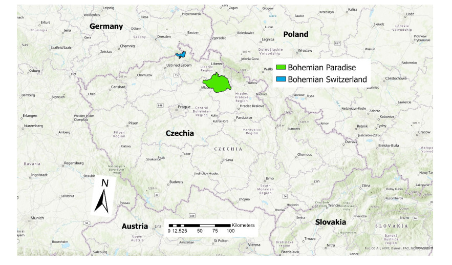
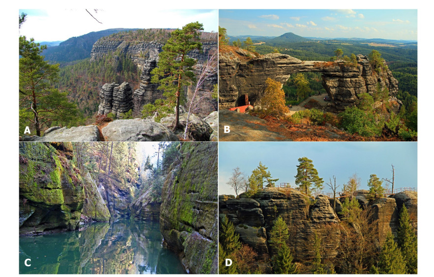
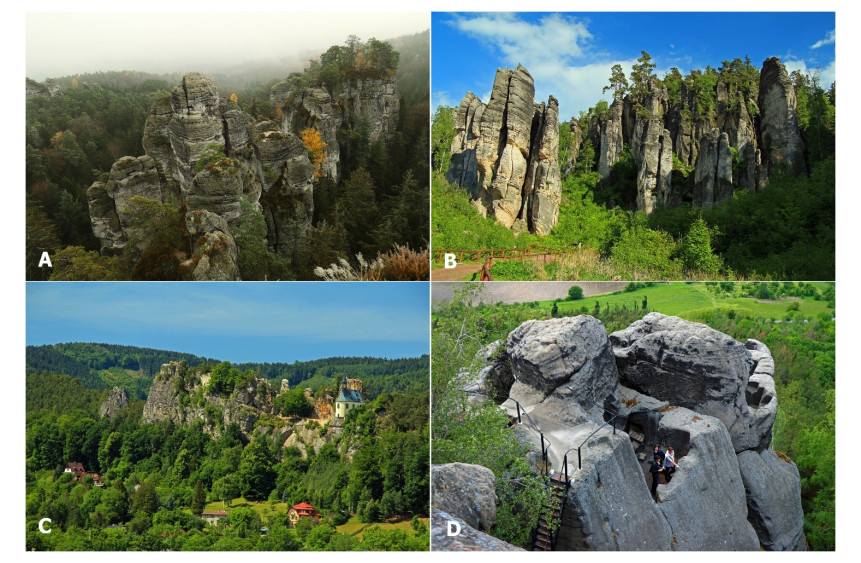
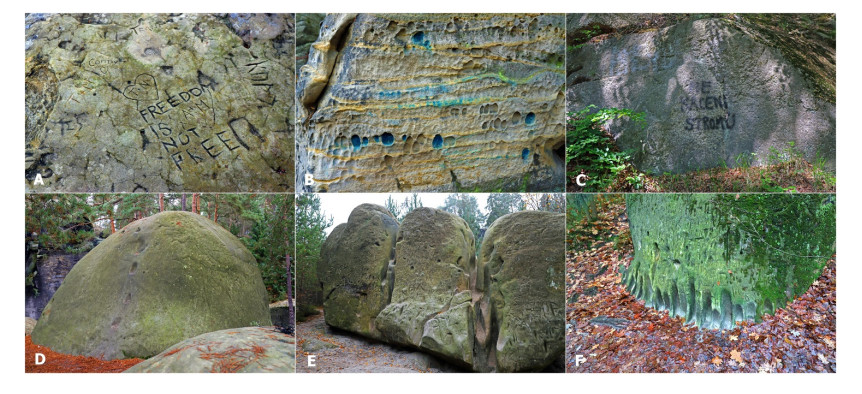
One of the most interesting natural tourist destinations in the Czech Republic are sandstone rocks, located mainly in the Bohemian Cretaceous Basin. Sandstones in these areas create a number of aesthetically valuable geomorphological formations, such as rock towers, gates, windows, overhangs etc. In addition, they provide beautiful views. Regions with a concentration of sandstone rocks are thus among the most visited natural areas in the Czech Republic. Unfortunately, mass tourism also brings negative impacts that negatively affect the condition of sandstone rocks—these are mainly engraving in the rocks, painting or spraying on the rocks, vandalism, pollution by garbage or excrements and destruction of natural rock shapes. However, it is not true that a larger number of visitors automatically means a larger number of negative impacts. This paper analyses the factors that influence the occurrence of the above-mentioned negative impacts in areas of sandstone rocks. The basis for the analysis was mapping of negative impacts in the field, data on traffic to individual geosites, GIS database of business entities in the tourism sector in the area of interest and field survey, aimed at explaining the structure of visitors to individual geosites according to their motivation and preferences. First, data on tourists' motivation and preferences were processed using cluster analysis into their typology. Then, the relationship between the intensity of the occurrence of negative impacts and potential factors—the absolute number of visitors, the distance to a major tourist facility and the type of visitor—was analysed. The results showed that damage to geosites is most affected by some types of visitors and little social control.

Keywords:

Citation: Emil Drápela. Prevention of damage to sandstone rocks in protected areas of nature in northern Bohemia[J]. AIMS Geosciences, 2021, 7(1): 56-73. doi: 10.3934/geosci.2021003

Related Papers:

[1]	Gonca Durmaz Güngör, Ishak Altun . Fixed point results for almost ( $\zeta -\theta _{\rho }$ )-contractions on quasi metric spaces and an application. AIMS Mathematics, 2024, 9(1): 763-774. doi: 10.3934/math.2024039
[2]	Hieu Doan . A new type of Kannan's fixed point theorem in strong $b$ - metric spaces. AIMS Mathematics, 2021, 6(7): 7895-7908. doi: 10.3934/math.2021458
[3]	Pragati Gautam, Vishnu Narayan Mishra, Rifaqat Ali, Swapnil Verma . Interpolative Chatterjea and cyclic Chatterjea contraction on quasi-partial $b$ -metric space. AIMS Mathematics, 2021, 6(2): 1727-1742. doi: 10.3934/math.2021103
[4]	Shaoyuan Xu, Yan Han, Suzana Aleksić, Stojan Radenović . Fixed point results for nonlinear contractions of Perov type in abstract metric spaces with applications. AIMS Mathematics, 2022, 7(8): 14895-14921. doi: 10.3934/math.2022817
[5]	Abdullah Shoaib, Poom Kumam, Shaif Saleh Alshoraify, Muhammad Arshad . Fixed point results in double controlled quasi metric type spaces. AIMS Mathematics, 2021, 6(2): 1851-1864. doi: 10.3934/math.2021112
[6]	Mi Zhou, Naeem Saleem, Xiao-lan Liu, Nihal Özgür . On two new contractions and discontinuity on fixed points. AIMS Mathematics, 2022, 7(2): 1628-1663. doi: 10.3934/math.2022095
[7]	Amjad Ali, Muhammad Arshad, Awais Asif, Ekrem Savas, Choonkil Park, Dong Yun Shin . On multivalued maps for $\varphi$ -contractions involving orbits with application. AIMS Mathematics, 2021, 6(7): 7532-7554. doi: 10.3934/math.2021440
[8]	Tahair Rasham, Abdullah Shoaib, Shaif Alshoraify, Choonkil Park, Jung Rye Lee . Study of multivalued fixed point problems for generalized contractions in double controlled dislocated quasi metric type spaces. AIMS Mathematics, 2022, 7(1): 1058-1073. doi: 10.3934/math.2022063
[9]	Xun Ge, Songlin Yang . Some fixed point results on generalized metric spaces. AIMS Mathematics, 2021, 6(2): 1769-1780. doi: 10.3934/math.2021106
[10]	Qing Yang, Chuanzhi Bai . Fixed point theorem for orthogonal contraction of Hardy-Rogers-type mapping on $O$ -complete metric spaces. AIMS Mathematics, 2020, 5(6): 5734-5742. doi: 10.3934/math.2020368

Abstract

1. Introduction

In various fields of science, nonlinear evolution equations practically model many natural, biological and engineering processes. For example, PDEs are very popular and are used in physics to study traveling wave solutions. They have played a crucial role in illustrating the nature of nonlinear problems. PDEs are collected to control the diffusion of chemical reactions. In biology, they play a fundamental role in describing various phenomena, such as population growth. In addition, natural phenomena such as fluid dynamics, plasma physics, optics and optical fibers, electromagnetism, quantum mechanics, ocean waves, and others are studied using PDEs. The qualitative and quantitative characteristics of these phenomena can be identified from the behaviors and shapes of their solutions. Therefore, finding the analytic solutions to such phenomena is a fundamental topic in mathematics. Scientists have developed sparse fundamental approaches to find analytic solutions for nonlinear PDEs. Among these techniques, I present integration methods from ^[1] and ^[2], the modified F-expansion and Generalized Algebraic methods, respectively. Bekir and Unsal ^[3] proposed the first integral method to find the analytical solution of nonlinear equations. Kumar, Seadawy and Joardar ^[4] used the improved Kudryashov technique to extract fractional differential equations. Adomian ^[5] proposed the Adomian decomposition technique to find the solution of frontier problems of physics. ^[6] uses an exploratory method to find explicit solutions of non-linear PDEs. Many different methods of solving equations arising from natural phenomena and some of their analytic solutions, such as dark and light solitons, non-local rogue waves, an occasional wave and mixed soliton solutions, are exhibited and can be found in ^{[7,8,9,10,11,12,13,14,15,16,17,18,19,20,21,22,23,24,25,26,27,28,29,30,31,32,33,34,35,36,37,38,39,40]}.

The Novikov-Veselov (NV) system ^[41,42] is given by

$\begin{equation} \begin{aligned} \Psi_t& +\alpha \Gamma_{xxy}+\beta \Phi_{xyy}+\gamma \Gamma_y \Phi+\gamma \left(\dfrac{\Psi^2}{2}\right)_y+\lambda\, \Gamma\, \Phi_x+\lambda\, \left(\dfrac{\Psi^2}{2}\right)_x = 0, \\ \Gamma_y& = \Psi_x, \\ \Psi_y& = \Phi_x, \\ \end{aligned} \end{equation}$

(1.1)

where $\alpha, \, \beta, \, \gamma$ and $\lambda$ are constants. Barman ^[42] declared that Eq (1.1) is involved to represent tidal and tsunami waves, electro-magnetic waves in communication cables and magneto-sound and ion waves in plasma. In ^[42], the generalized Kudryashov method was utilized to have traveling wave solutions for Eq (1.1). According to Croke ^[43], the Novikov-Veselov system is generalized from the KdV equations which were examined by Novikov and Veselov. Croke ^[43] used several approaches, (the extended mapping, the Hirota and the extended tanh-function approaches) in the proposed system to achieve numerous soliton solutions, such as breathers, and constrained analytic solutions. Boiti, Leon, and Manna ^[44] applied the inverse dispersion technique to solve (1.1) for a particular type of initial value. Numerical solutions and a study of the stability of solutions for the proposed equation were presented by Kazeykina and Klein ^[45]. The Nizhnik-Novikov-Veselov system for two dimensions was also solved using the Kansa technique to find the numerical results ^[46]. To the best of my knowledge, the stability and error analysis of the numerical scheme presented here has not yet been discussed for system (1.1). Therefore, this has motivated me enormously to do so. The primary purpose is to obtain multiple analytic solutions to system (1.1) by using both the modified F-expansion and Generalized Algebraic methods. In connection with the numerical solution, the method of finite differences is utilized to achieve numerical results for the studied system. I graphically and analytically compare the traveling wave solutions and numerical results. Undoubtedly, the presented results strongly contribute to describing physical problems in practice.

The outline of this article is provided in this paragraph. Section 2 summarizes the employed methods. All the analytic solutions are extracted in Section 3. The shooting and BVP results for the proposed system are presented in Section 4. In addition, I examine the numerical solution of the system (1.1) in Section 5. Sections 6 and 7 study the stability and error analysis of the numerical scheme, respectively. Section 8 presents the results and discussion.

2. Summary of proposed methods

Considering the development equation with physical fields $\Psi(x, y, t)$ , $\Phi(x, y, t)$ and $\Gamma(x, y, t)$ in the variables $x,$ $y$ and $t$ is given in the following form:

$\begin{equation} Q_1(\Psi, \Psi_t, \Psi_x, \Psi_y, \Gamma, \Gamma_y, \Gamma_{xxy}, \Phi, \Phi_{xyy}, \Phi_{x}, \dots) = 0. \end{equation}$

(2.1)

Step 1. We extract the traveling-wave solutions of System (1.1) that are formed as follows:

$\begin{equation} \begin{aligned} \Phi(x, y, t) = &\phi(\eta) , &&\qquad&\eta = x+y-wt, \\ \Psi(x, y, t) = &\psi(\eta), \\ \Gamma(x, y, t) = &\Theta(\eta), \end{aligned} \end{equation}$

(2.2)

where $w$ is the wave speed.

Step 2. The nonlinear evolution (2.1) is reduced to the following ODE:

$\begin{equation} Q_2(\psi, \psi_\eta, \Theta, \Theta_\eta, \Theta_{\eta\eta\eta}, \phi, \phi_{\eta\eta\eta}, \phi_{\eta}, \dots) = 0, \end{equation}$

(2.3)

where $Q_2$ is a polynomial in $\psi(\eta), \; \phi(\eta),$ $\Theta(\eta)$ and their total derivatives.

2.1. The modified F-expansion method

According to the modified F-expansion method, the solutions of (2.3) are given by the form

$\begin{equation} \psi(\eta) = \rho_0+\sum\limits_{k = 1}^{N} \left( \rho_{k} F(\eta)^{k}+\dfrac{ q_{k}}{F(\eta)^{k}} \right) , \end{equation}$

(2.4)

and $F(\eta)$ is a solution of the following differential equation:

$\begin{equation} F^{\prime}(\eta) = \mu_0+\mu_1 F(\eta)+\mu_2 F(\eta)^{2}, \end{equation}$

(2.5)

where $\mu_0$ , $\mu_1$ , $\mu_2$ , are given in ^[1], and $\rho_k$ , $q_k$ are to be determined later.

Table 1. The relations among

$\mu_0$ ,

$\mu_1$ ,

$\mu_2$ and the function

$F(\eta)$ .

$\mu_0$	$\mu_{1}$	$\mu_{2}$	$F(\eta)$
$\mu_0=0,$	$\mu_1=1,$	$\mu_2=-1,$	$F(\eta)=\dfrac{1}{2}+\dfrac{1}{2} \tanh \left(\dfrac{1}{2} \eta\right).$
$\mu_0=0,$	$\mu_1=-1,$	$\mu_2=1,$	$F(\eta)=\dfrac{1}{2}-\dfrac{1}{2} \operatorname{coth}\left(\dfrac{1}{2} \eta\right).$
$\mu_0=\dfrac{1}{2},$	$\mu_1=0,$	$\mu_2=\dfrac{-1}{2},$	$F(\eta)=\operatorname{coth}(\eta) \pm \operatorname{csch}(\eta),$ $\tanh (\eta) \pm \operatorname{sech}(\eta).$
$\mu_0=1,$	$\mu_1=0,$	$\mu_2=-1,$	$F(\eta)=\tanh (\eta),$ $\operatorname{coth}(\eta).$
$\mu_0=\dfrac{1}{2},$	$\mu_1=0,$	$\mu_2=\dfrac{1}{2},$	$F(\eta)=\sec (\eta)+\tan (\eta),$ $\csc (\eta)-\cot (\eta).$
$\mu_0=\dfrac{1}{2},$	$\mu_1=0,$	$\mu_2=\dfrac{1}{2},$	$F(\eta)=\sec (\eta)-\tan (\eta),$ $\csc (\eta)+\cot (\eta).$
$\mu_0=\pm1,$	$\mu_1=0,$	$\mu_2=\pm1,$	$F(\eta)=\tan (\eta),$ $\cot (\eta).$

| Show Table

DownLoad: CSV

2.2. The generalized algebraic method

According to the generalized direct algebraic method, the solutions of (2.3) are given by

$\begin{equation} \psi(\eta) = \nu_0+\sum\limits_{k = 1}^{N} \left( \nu_{k} G(\eta)^{k} +\dfrac{ r_{k}}{G(\eta) ^{k}} \right) , \end{equation}$

(2.6)

and $G(\eta)$ is a solution of the following differential equation:

$\begin{equation} G^{\prime}(\eta) = \varepsilon \sqrt{\sum\limits_{k = 0}^{4} \delta_{k} G^{k}(\eta)}, \end{equation}$

(2.7)

where $\nu_k,$ and $r_k$ are to be determined, and $N$ is an integer number obtained by the highest degree of the nonlinear terms and the highest order of the derivatives. $\varepsilon$ is user-specified, usually taken with $\varepsilon = \pm1$ , and $\delta_k$ , $k = 0, 1, 2, 3, 4,$ are given in Table 2 ^[2].

Table 2. The relations among

$\delta_k$ ,

$k = 0, 1, 2, 3, 4,$ and the function

$G(\eta)$ .

$\delta_{0}$	$\delta_{1}$	$\delta_{2}$	$\delta_{3}$	$\delta_{4}$	$G(\eta)$
$\delta_{0}=0$ ,	$\delta_{1}=0$ ,	$\delta_{2} > 0$ ,	$\delta_{3}=0$ ,	$\delta_{4} < 0$ ,	$G(\eta)= \varepsilon$ $\sqrt{-\dfrac{\delta_{2}}{\delta_{4}}} \operatorname{sech}\left(\sqrt{\delta_{2}} \eta\right)$ .
$\delta_{0}=\dfrac{\delta_{2}^{2}}{4 c 4}$ ,	$\delta_{1}=0$ ,	$\delta_{2} < 0$ ,	$\delta_{3}=0$ ,	$\delta_{4} > 0$ ,	$G(\eta)=\varepsilon \sqrt{-\dfrac{\delta_{2}}{2 \delta_{4}}} \tanh \left(\sqrt{-\dfrac{\delta_{2}}{2}} \eta\right)$ .
$\delta_{0}=0$ ,	$\delta_{1}=0$ ,	$\delta_{2} < 0$ ,	$\delta_{3}=0$ ,	$\delta_{4} > 0$ ,	$G(\eta)=\varepsilon$ $\sqrt{-\dfrac{\delta_{2}}{\delta_{4}}}$ $\sec$ $\left(\sqrt{-\delta_{2}} \eta\right)$ .
$\delta_{0}=\dfrac{\delta_{2}^{2}}{4 \delta_{4}},$	$\delta_{1}=0$ ,	$\delta_{2} > 0$ ,	$\delta_{3}=0,$	$\delta_{4} > 0,$	$G(\eta)=\varepsilon$ $\sqrt{\dfrac{\delta_{2}}{2 \delta_{4}}} \tan \left(\sqrt{\dfrac{\delta_{2}}{2}} \eta\right)$ .
$\delta_{0}=0,$	$\delta_{1}=0,$	$\delta_{2}=0,$	$\delta_{3}=0,$	$\delta_{4} > 0,$	$G(\eta)=-\dfrac{\varepsilon}{\sqrt{\delta_{4}} \eta}$ .
$\delta_{0}=0,$	$\delta_{1}=0,$	$\delta_{2} > 0,$	$\delta_{3}\neq 0,$	$\delta_{4}=0,$	$G(\eta)=-\dfrac{\delta_{2}}{\delta_{3}}. \operatorname{sech}^{2}\left(\dfrac{\sqrt{\delta_{2}}}{2} \eta\right)$ .

| Show Table

DownLoad: CSV

3. Methodology

Consider the Novikov-Veselov (NV) system

(3.1)

a system of PDEs in the unknown functions $\Psi = \Psi(x, y, t), \; \Phi = \Phi(x, y, t)$ , $\Gamma = \Gamma(x, y, t)$ and their partial derivatives. I plug the transformations

$\begin{equation} \begin{aligned} \Phi(x, y, t) = &\phi(\eta) , &&\qquad&\eta = x+y-wt, \\ \Psi(x, y, t) = &\psi(\eta), \\ \Gamma(x, y, t) = &\Theta(\eta), \end{aligned} \end{equation}$

(3.2)

into Eq (3.1) to reduce it to a system of ODEs given by

$\begin{equation} \begin{aligned} -w\; \psi_\eta& +\alpha \Theta_{\eta\eta\eta}+\beta \phi_{\eta\eta\eta}+\gamma \Theta_\eta \phi+\gamma \left(\dfrac{\psi^2}{2}\right)_\eta+\lambda\, \Theta\, \phi_\eta+\lambda\, \left(\dfrac{\psi^2}{2}\right)_\eta = 0, \\ \Theta_\eta& = \psi_\eta, \\ \psi_\eta& = \phi_\eta.\\ \end{aligned} \end{equation}$

(3.3)

Integrating $\Theta_\eta = \psi_\eta$ and $\phi_\eta = \psi_\eta$ yields

$\begin{equation} \Theta = \psi, \qquad \text{and } \qquad \phi = \psi. \end{equation}$

(3.4)

Substituting (3.4) into the first equation of (3.3) and integrating once with respect to $\eta$ yields

$\begin{equation} \begin{aligned} -w\; \psi& +\left( \alpha +\beta\right) \psi_{\eta\eta}+\left( \gamma+\lambda\right) \psi^2 = 0. \end{aligned} \end{equation}$

(3.5)

Balancing $\psi_{\eta\eta}$ with $\psi^2$ in (3.5) calculates the value of $N = 2.$

3.1. Application of modified F-expansion method

According to the modified F-expansion method with $N = 2$ , the solutions of (3.5) are

$\begin{equation} \psi(\eta) = \rho_0+ \rho_{1} F(\eta)+\dfrac{ q_{1}}{F(\eta)}+ \rho_{2} F(\eta)^{2}+\dfrac{ q_{2}}{F(\eta)^{2}} , \end{equation}$

(3.6)

and $F(\eta)$ is a solution of the following differential equation:

$\begin{equation} F^{\prime}(\eta) = \mu_0+\mu_1 F(\eta)+\mu_2 F(\eta)^{2}, \end{equation}$

(3.7)

where $\mu_0$ , $\mu_1$ , $\mu_2$ are given in Table 1. To explore the analytic solutions to (3.5), I ought to follow the subsequent steps.

$\textbf{Step 1.}$ Placing (3.6) along with (3.7) into Eq (3.5) and gathering the coefficients of $F(\eta)^j$ , $j$ = $-4, -3, -2, -1, 0, 1, 2, 3, 4,$ to zeros gives a system of equations for $\rho_0, \; \rho_k, \; q_k$ , $k = 1, 2.$

$\textbf{Step 2.}$ Solve the resulting system using mathematical software: for example, Mathematica or Maple.

$\textbf{Step 3.}$ Choosing the values of $\mu_0, \; \mu_1$ and $\mu_2$ and the function $F(\eta)$ from and substituting them along with $\rho_0, \; \rho_k, \; q_k$ , $k = 1, 2,$ in (3.6) produces a set of trigonometric function and rational solutions to (3.5).

Applying the above steps, I determine the values of $\rho_0, \; \rho_1, \; \rho_2, \; q_1, \; q_2$ and $w$ as follows:

$(1).$ When $\mu_0 = 0,$ $\mu_1 = 1$ and $\mu_2 = -1$ , I have two cases.

$\textbf{Case 1.}$

$\begin{equation} \begin{aligned} \rho_0 = &0, && \rho_1 = \dfrac{6 (\alpha +\beta)}{\gamma +\lambda}, &\rho_2 = & -\dfrac{6 (\alpha +\beta)}{\gamma + \lambda}, & q_1 = q_2 = 0, \quad \text{and}\quad w = \alpha+\beta. \end{aligned} \end{equation}$

(3.8)

The solution is given by

$\begin{equation} \begin{aligned} \Psi_1(x, y, t) = \dfrac{ 3(\alpha+\beta)}{2(\gamma+\lambda)} \operatorname{sech}^2\left(\dfrac{1}{2} \left( x+y-(\alpha +\beta) t+x0\right) \right). \end{aligned} \end{equation}$

(3.9)

$\textbf{Case 2.}$

$\rho_0 = -\dfrac{\alpha+\beta}{\gamma+\lambda}, \rho_1 = \dfrac{6 (\alpha +\beta)}{\gamma +\lambda}, \\ \rho_2 = -\dfrac{6 (\alpha +\beta)}{\gamma + \lambda}, q_1 = q_2 = 0, \quad \text{and}\quad w = -\left( \alpha+\beta\right) .$

(3.10)

The solution is given by

$\begin{equation} \begin{aligned} \Psi_2(x, y, t) = -\dfrac{ (\alpha+\beta)}{2(\gamma+\lambda)} \left( 3 \tanh ^2\left(\dfrac{1}{2} (x+y+t (\alpha+\beta))+x0\right)-1 \right) . \end{aligned} \end{equation}$

(3.11)

presents the time evolution of the analytic solutions $(a)$ $\Psi_1$ and $(b)$ $\Psi_2$ with $t = 0, 10, 20$ . The parameter values are $x0 = -20, \ \alpha = 0.50, \beta = 0.6, \ \gamma = -1.5,$ and $\lambda = 1.$ presents the wave behavior by changing a certain parameter value and fixing the values of the others. presents the behavior of $\Psi_1$ when I change the values of (a) $\alpha$ or $\beta$ and (b) $\gamma$ or $\lambda$ . In it can also be seen that the value of $\alpha$ or $\beta$ affects the direction and amplitude of the wave, such that a negative value always makes the wave negative, its amplitude decreases when $\alpha, \, \beta \to 0$ , and its amplitude increases when $\alpha, \, \beta \to \infty.$ In the value of $\gamma$ or $\lambda$ affects the direction and amplitude of the wave, such that a negative value always makes the wave negative, and its amplitude decreases when the value of $\gamma$ or $\lambda$ increases. In and present the wave behavior of $\Psi_2.$

Figure 1. Time evolution of the analytic solutions

$(a)$

$\Psi_1$ and

$(b)$

$\Psi_2$ with

$t = 0, 10, 20$ . The parameter are given by

$x0 = -20, \ \alpha = 0.50, \beta = 0.6, \ \gamma = -1.5,$ and

$\lambda = 1$ .

DownLoad: Full-Size Img PowerPoint

Figure 2. This figure present the wave behavior when changing a certain parameter value and fixing the values of the others.

$(a)$ presents the behavior when I change the value of

$\alpha$ or

$\beta,$ and

$(b)$ presents when I change the value of

$\gamma$ or

$\lambda$ for the solution

$\Psi_1.$

$(c)$ and

$(d)$ are for

$\Psi_2$ .

DownLoad: Full-Size Img PowerPoint

$(2).$ When $\mu_0 = 0,$ $\mu_1 = -1,$ and $\mu_2 = 1$ , I have two cases.

$\textbf{Case 3.}$ The solution is given by

$\begin{equation} \begin{aligned} \Psi_3(x, y, t) = -\dfrac{ 3(\alpha+\beta)}{2(\gamma+\lambda)} \operatorname{csch}^2\left(\dfrac{1}{2} \left( x+y-(\alpha +\beta) t\right) \right). \end{aligned} \end{equation}$

(3.12)

$\textbf{Case 4.}$ The solution is given by

$\begin{equation} \begin{aligned} \Psi_4(x, y, t) = -\dfrac{ (\alpha+\beta)}{2(\gamma+\lambda)} \left( 3 \coth ^2\left(\dfrac{1}{2} (x+y+t (\alpha+\beta))\right)-1 \right) . \end{aligned} \end{equation}$

(3.13)

$(3).$ When $\mu_0 = 1,$ $\mu_1 = 0,$ and $\mu_2 = -1$ , I have

$\textbf{Case 5.}$ The solution is given by

$\begin{equation} \begin{aligned} \Psi_5(x, y, t) = -\dfrac{8 (\alpha+\beta) }{\gamma+\lambda}(\cosh (4 (16 t (\alpha+\beta)+x+y))+2) \operatorname{csch}^2(2 (16 t (\alpha+\beta)+x+y)). \end{aligned} \end{equation}$

(3.14)

$(4).$ When $\mu_0 = \pm 1,$ $\mu_1 = 0,$ and $\mu_2 = \pm 1$ , I have one case.

$\textbf{Case 6.}$ The solution is given by

$\begin{equation} \begin{aligned} \Psi_6(x, y, t) = -\dfrac{24 (\alpha+\beta) }{\gamma+\lambda}\csc ^2(2 (16 t (\alpha+\beta)+x+y)) . \end{aligned} \end{equation}$

(3.15)

3.2. Application of the generalized algebraic method

According to the generalized algebraic method, the solutions of (3.5) are given by the form

$\begin{equation} \psi(\eta) = \nu_0+ \nu_{1} G(\eta)+ \nu_{2} G(\eta)^{2}+\dfrac{ r_{1}}{G(\eta)}+\dfrac{ r_{2}}{G(\eta)^{2}}, \end{equation}$

(3.16)

where $\nu_k$ , $r_k$ are to be determined later. $G(\eta)$ is a solution of the following differential equation:

$\begin{equation} G^{\prime}(\eta) = \varepsilon \sqrt{\sum\limits_{k = 0}^{4} \delta_{k} G^{k}(\eta)}, \end{equation}$

(3.17)

where $\delta_k$ , $k = 0, 1, 3, 4$ , are given in . In all the cases mentioned above and the subsequent solutions, I used the mathematical software Mathematica to find the values of the constants $\nu_0, \, \nu_1, \, \nu_2, \, r_1, \, r_2$ and $w$ . Thus, the analytic solutions to (3.5) using the generalized algebraic method will be presented here with different values of the constants $\delta_k$ , $k = 0, 1, 3, 4$ .

$(5).$ When $\delta_0 = \dfrac{\delta^2_2}{4 \delta_4},$ $\delta_1 = \delta_3 = 0,$ $\delta_2 < 0$ , $\delta_4 > 0$ , and $\varepsilon = \pm1,$

$\begin{equation} \begin{aligned} \nu_0 = &\frac{\pm\sqrt{4 \delta_2^2 \varepsilon^4 \left(\alpha+\beta\right)^2 \left(\gamma+\lambda\right)^2-3 \delta_2 \varepsilon^4 \left(\alpha+\beta\right)^2 \left(\gamma+\lambda\right)^2}-2 \delta_2 \varepsilon^2 \left(\alpha+\beta\right) \left(\gamma+\lambda\right)}{\left(\gamma+\lambda\right)^2}, \\ \nu_2 = &-\frac{6 \delta_4 \varepsilon^2 \left(\alpha+\beta\right)}{\left(\gamma+\lambda\right)}, \\ \nu_1 = &r_1 = r_2 = 0, \quad\varepsilon = \pm1.\\ w = &\pm\frac{2 \sqrt{\left(4 \delta_2^2-3 \delta_2\right) \varepsilon^4 \left(\alpha+\beta\right)^2 \left(\gamma+\lambda\right)^2}}{\left(\gamma+\lambda\right)}. \end{aligned} \end{equation}$

(3.18)

$\textbf{Case 7.}$ The solution is given by

$\Psi_7(x, y, t) = -\frac{1}{{(\gamma+\lambda)^2}}\\ \left( -3 \delta_2 \varepsilon^4 (\alpha+\beta) (\gamma+\lambda) \tanh ^2\left(\frac{\sqrt{-\delta_2} \left(\frac{2 t \sqrt{\delta_2 (4 \delta_2-3) \varepsilon^4 (\alpha+\beta)^2 (\gamma+\lambda)^2}}{\gamma+\lambda}+x+y\right)}{\sqrt{2}}\right)\right.\\ \left.+2 \delta_2 \varepsilon^2 (\alpha+\beta) (\gamma+\lambda)+\sqrt{\delta_2 (4 \delta_2-3) \varepsilon^4 (\alpha+\beta)^2 (\gamma+\lambda)^2}\right) .$

(3.19)

shows the time evolution of the analytic solutions. shows $\Psi_7$ with $t$ = $0:2:6$ . The parameter values are $\delta_2 = -1$ , $\delta_4 = 1,$ $\epsilon = -1,$ $\alpha = 0.50,$ $\beta = 0.6,$ $\gamma = -1.5,$ $\lambda = 1.8$ and $x0 = -10.$ shows $\Psi_8$ with $t = 0:2:8$ . The parameter values are $\delta_2 = 1$ , $\delta_4 = -1,$ $\epsilon = -1,$ $\alpha = 0.50,$ $\beta = 0.6,$ $\gamma = -1.5,$ $\lambda = 1.8$ and $x0 = -10.$ – present the $3D$ time evolution of the analytic solutions $\Psi_2$ (left) and the numerical solutions (right) obtained employing the scheme 5.1 with $t = 5, 15, 25$ , $M_x = 1600,$ $N_y = 100,$ $x = 0\to60$ and $y = 0\to1.$

Figure 3. Time evolution of the analytic solutions.

$(a)$

$\Psi_7$ with

$t = 0:2:6$ . The parameter values are

$\delta_2 = -1$ ,

$\delta_4 = 1,$

$\epsilon = -1,$

$\alpha = 0.50,$

$\beta = 0.6,$

$\gamma = -1.5,$

$\lambda = 1.8$ and

$x0 = -10.$

$(b)$

$\Psi_8$ with

$t = 0:2:8$ . The parameter values are

$\delta_2 = 1$ ,

$\delta_4 = -1,$

$\epsilon = -1,$

$\alpha = 0.50,$

$\beta = 0.6,$

$\gamma = -1.5,$

$\lambda = 1.8$ and

$x0 = -10$ .

DownLoad: Full-Size Img PowerPoint

Figure 4. 3D graphs presenting the analytic (left) and the numerical (right) solutions of

$\Psi_2(x, y, t)$ at

$t = 5.$ The figures present the strength of agreement between analytic and numerical solutions.

DownLoad: Full-Size Img PowerPoint

Figure 5. 3D graphs presenting the analytic (left) and the numerical (right) solutions of

$\Psi_2(x, y, t)$ at

$t = 15.$ The figures present the strength of agreement between analytic and numerical solutions.

DownLoad: Full-Size Img PowerPoint

Figure 6. 3D graphs presenting the analytic (left) and the numerical (right) solutions of

$\Psi_2(x, y, t)$ at

$t = 25.$ The figures present the strength of agreement between analytic and numerical solutions.

DownLoad: Full-Size Img PowerPoint

$(6).$ When $\delta_0 = 0,$ $\delta_1 = \delta_3 = 0,$ $\delta_2 > 0$ , $\delta_4 < 0$ , and $\varepsilon = \pm1,$

$\begin{equation} \begin{aligned} \nu_2 = &-\frac{6 \delta_4 \varepsilon^2 (\alpha+\beta)}{\gamma+\lambda}, \quad \nu_1 = \nu_0 = r_1 = r_2 = 0, \quad w = &4 \delta_2 \varepsilon^2 (\alpha+\beta). \end{aligned} \end{equation}$

(3.20)

$\textbf{Case 8.}$ The solution is given by

$\begin{equation} \begin{aligned} \Psi_8(x, y, t) = &\frac{6 \delta_2\epsilon^4 (\alpha+\beta) \operatorname{sech}^2\left(\sqrt{\delta_2} \left(-4 \delta_2\epsilon^2 t (\alpha+\beta)+x+y\right)\right)}{\gamma+\lambda} \end{aligned} \end{equation}$

(3.21)

$(7).$ When $\delta_0 = 0,$ $\delta_1 = \delta_4 = 0,$ $\delta_3\neq0,$ $\delta_2 > 0$ , $\varepsilon = \pm1$

$\begin{equation} \begin{aligned} \text{Set 1.}\, \nu_1 = & -\tfrac{3 \delta_3 \varepsilon^2 \left(\alpha+\beta\right)}{2 \left(\gamma+\lambda\right)}, \, \nu_0 = \nu_2 = r_1 = r_2 = 0, \, w = \delta_2 \varepsilon^2 \left(\alpha+\beta\right). \\ &\\ \text{Set 2.}\, \nu_0 = & -\tfrac{\delta_2 \varepsilon^2 \left(\alpha+\beta\right)}{\left(\gamma+\lambda\right)}, \, \nu_1 = -\tfrac{3 \delta_3 \varepsilon^2 \left(\alpha+\beta\right)}{2 \left(\gamma+\lambda\right)}, \quad\nu_2 = r_1 = r_2 = 0, \, w = -\delta_2 \varepsilon^2 \left(\alpha+\beta\right). \end{aligned} \end{equation}$

(3.22)

$\textbf{Case 9.}$ The solution is given by

$\begin{equation} \begin{aligned} \Psi_9(x, y, t) = \frac{3 \delta_2 (\alpha+\beta) \operatorname{sech}^2\left(\frac{1}{2} \sqrt{\delta_2} (\delta_2 t (-(\alpha+\beta))+x+y)\right)}{2 (\gamma+\lambda)}. \end{aligned} \end{equation}$

(3.23)

$\textbf{Case 10.}$ The solution is given by

$\begin{equation} \begin{aligned} \Psi_{10}(x, y, t) = \frac{3 \delta_2 (\alpha+\beta) \operatorname{sech}^2\left(\frac{1}{2} \sqrt{\delta_2} (\delta_2 t (\alpha+\beta)+x+y)\right)}{2 (\gamma+\lambda)}-\frac{\delta_2 (\alpha+\beta)}{\gamma+\lambda}. \end{aligned} \end{equation}$

(3.24)

4. Numerical solution

In this section I extract numerical solutions to the resulting ODE system (3.5) using several numerical methods. The purpose of this procedure is to guarantee the accuracy of the analytic solutions. I picked one of the analytic solutions above to be a sample, (3.11). The nonlinear shooting and BVP methods, at $t = 0,$ are used by taking the value of $\psi$ at the right endpoint of the domain $\eta = 0$ with guessing the initial value for $\psi_\eta.$ The new target is to obtain the second boundary condition of $\psi$ at the left endpoint of a particular domain. Once the numerical result is obtained, I compare it with the analytic solution (3.11). The MATLAB solver ODE15s and FSOLVE ^[47] are used to get the numerical solution. The resulting ODE (3.5) is discretized as

$\begin{equation} f(\psi) = 0, \qquad f(\psi_i) = -w\; \psi_i +\dfrac{\alpha +\beta}{\Delta_\eta} \left( \psi_{i+1}-2\psi_i+\psi_{i-1}\right) +\dfrac{ \gamma+\lambda}{2\Delta_\eta} \left( \psi^2_{i+1}-\psi_{i-1}^2\right), \end{equation}$

(4.1)

for the BVP method and

$\begin{equation} \psi_{\eta\eta} = \dfrac{1}{\alpha+\beta}\left( w\psi-\left( \gamma+\lambda\right) \psi^2\right), \end{equation}$

(4.2)

for the shooting method. Figure 7 presents the comparison between the numerical solutions obtained using the above numerical methods and the analytic solution. Figure 7 shows that the solutions are identical to the analytic solution.

Figure 7. Comparing the numerical solutions resulting from the shooting and BVP methods with the analytic solution (3.11) at

$t = 0.$ The parameter values are taken as

$\alpha = 0.50$ ,

$\beta = 0.6$ ,

$\gamma = -1.5, \lambda = 1.8$ , with

$N = 600$ .

DownLoad: Full-Size Img PowerPoint

Thus, it is possible to verify the correctness of the analytic solution. I also accept the obtained numerical solution as an initial condition for the numerical scheme in the next section.

5. Numerical scheme on a fixed mesh

In this section, I use the finite-difference method to obtain the numerical results of system (1.1) over the domain $[a, \, b]\times [c, \, d].$ Here, $a, \; b, \; c$ and $d$ represent the endpoints of the rectangular domain in the $x$ and $y$ directions, respectively, and $T_f$ is a certain time. The domain $[a, \, b]\times [c, \, d]$ is split into $(M_x+1)\times (N_y+1)$ mesh points:

$\begin{equation*} \label{} \begin{aligned} x_m = &a+m\, \Delta_x, &&& m = 0, \, 1, \, 2, \, \dots, \, M_x, \\ y_n& = c+n\, \Delta_y, &&& n = 0, \, 1, \, 2, \, \dots, \, N_y, \end{aligned} \end{equation*}$

where $\Delta_x$ and $\Delta_y$ are the step-sizes of the $x$ and $y$ domains, respectively. The system (1.1) is converted to an ODE system by discretizing the space derivatives while keeping the time derivative continuous. Completing this yields

$\begin{equation} \begin{aligned} &\Psi_t|_{m, n}^k + \dfrac{\alpha}{2\Delta_y \Delta_x^2} \delta_x^2\left( \Gamma^{k+1}_{m, n+1}-\Gamma^{k+1}_{m, n-1}\right) +\dfrac{\beta}{2\Delta_x\Delta_y^2} \delta_y^2\left( \Phi^{k+1}_{m+1, n}-\Phi^{k+1}_{m-1, n}\right)\\ &\qquad \quad- \frac{ \gamma}{4\Delta_y} \left( \left( \Phi^{k+1}_{m, n+1}+\Phi^{k+1}_{m, n} \right) \Gamma^{k+1}_{m, n+1}- \left( \Phi^{k+1}_{m, n}+\Phi^{k+1}_{m, n-1} \right)\Gamma^{k+1}_{m, n-1}\right)\\ &\qquad \quad- \frac{ \lambda}{4\Delta_x} \left( \left( \Gamma^{k+1}_{m+1, n}+\Gamma^{k+1}_{m, n} \right) \Phi^{k+1}_{m+1, n}- \left( \Gamma^{k+1}_{m, n}+\Gamma^{k+1}_{m-1, n} \right)\Phi^{k+1}_{m-1, n}\right)\\ &\qquad \quad+\frac{ \gamma}{4\Delta_y} \left( \left( \Psi^{k+1}_{m, n+1}\right)^2- \left( \Psi^{k+1}_{m, n-1}\right)^2\right) +\frac{ \lambda}{4\Delta_x} \left( \left( \Psi^{k+1}_{m+1, n}\right)^2- \left( \Psi^{k+1}_{m-1, n}\right)^2\right) = 0, \\ &\frac{1}{2\Delta_y}(\Gamma_{m, n+1}^{k+1}-\Gamma_{m, n-1}^{k+1}) = \frac{1}{2\Delta_x}(\Psi_{m+1, n}^{k+1}-\Psi_{m-1, n}^{k+1}), \\ &\frac{1}{2\Delta_y}(\Psi_{m, n+1}^{k+1}-\Psi_{m, n-1}^{k+1}) = \frac{1}{2\Delta_x}(\Phi_{m+1, n}^{k+1}-\Phi_{m-1, n}^{k+1}), \end{aligned} \end{equation}$

(5.1)

where

$\begin{aligned} \delta_x^2\Gamma_{m, n}^{k+1} = &\left(\Gamma^{k+1}_{m+1, n}-2 \Gamma^{k+1}_{m, n}+ \Gamma^{k+1}_{m-1, n}\right), \\ \delta_y^2\Phi_{m, n}^{k+1} = &\left(\Phi^{k+1}_{m, n+1}-2 \Phi^{k+1}_{m, n}+ \Phi^{k+1}_{m, n-1}\right), \end{aligned}$

subject to the boundary conditions:

$\begin{equation} \begin{array}{l} \Psi_{x}(a, \, y, \, t) = \Psi_{x}(b, \, y, \, t) = 0, \, \, \, \, \, \, \, \, \forall y\in [c, \, d], \\ \\ \Psi_{y}(x, \, c, \, t) = \Psi_{y}(x, \, d, \, t) = 0, \, \, \, \, \, \forall x\in [a, \, b]. \end{array} \end{equation}$

(5.2)

Equation (5.2) permits us to use fictitious points in estimating the space derivatives at the domain's endpoints. The initial conditions are generated by

$\begin{equation} \begin{aligned} \Psi_2(x, y, 0) = -\dfrac{ (\alpha+\beta)}{2(\gamma+\lambda)} \left( 3 \tanh ^2\left(\dfrac{1}{2} (x+y+x0\right)-1 \right) , \end{aligned} \end{equation}$

(5.3)

where $\alpha, \, \beta, \, \gamma$ and $\lambda$ are user-defined parameters. In all the numerical results shown in this section, the parameter values are fixed as $\alpha = 0.50, \, \beta = 0.6, \, \gamma = -1.50, \, \lambda = 1.80, \, x0 = -45.0$ , $y = 0\to1,$ $x = 0\to60$ and $t = 0\to 25.$ The above system is solved by using an ODE solver in FORTRAN called the DDASPK solver ^[48]. This solver used a backward differentiation formula. Since I do not have the initial conditions for the space derivatives, I approximate the Jacobian matrix of the linearized system by using LU-Factorization. The obtained numerical results are acceptable. This can be observed from the Figures 8 and 9.

Figure 8. Time change for the numerical results while holding

$y = 0.5$ and

$M_x = 1600$ at

$t = 0:5:25.$ The wave at

$t = 25$ illustrates that the numerical and the analytic solutions are quite identical.

DownLoad: Full-Size Img PowerPoint

Figure 9. The convergence histories of the scheme with the fixation of both

$y = 0.5$ and

$M_x = 1600$ at

$t = 5$ .

DownLoad: Full-Size Img PowerPoint

6. Stability of the numerical scheme

The von Neumann analysis is used to examine the stability of the scheme (5.1). The von Neumann analysis is occasionally called Fourier analysis and is utilized exclusively when the scheme is linear. Hence, I suppose that the linear version is given by

$\begin{equation} \begin{aligned} \Psi_t& +\alpha \Gamma_{xxy}+\beta \Phi_{xyy}+s_0\, \Gamma_y+s_1\, \Psi_y+s_2\, \Phi_x+s_3\, \Psi_x = 0, \\ \Gamma_y& = \Psi_x, \\ \Psi_y& = \Phi_x, \\ \end{aligned} \end{equation}$

(6.1)

where $s_0 = \gamma \Phi$ , $s_1 = \gamma \Psi$ , $s_2 = \lambda \Gamma$ , $s_3 = \lambda \Psi$ are constants. Since $\Gamma_y = \Psi_x,$ and $\Psi_y = \Phi_x,$ the first equation of (6.1) is given by

$\begin{equation} \Psi_t +\alpha \Psi_{xxx}+\beta \Psi_{yyy}+ s_0\, \Psi_y +s_1\, \Psi_y+s_2\, \Psi_x+s_3\, \Psi_x = 0, \end{equation}$

(6.2)

where $\alpha, \, \beta, \, \gamma, \, \lambda, \, s_0, \, s_1, \, s_2, \, s_3, \, l_4$ are constants. I set directly

$\begin{equation} \begin{aligned} \Psi_{m, n}^k = &\mu^k\, \exp(\iota\, \pi\, \xi_0 \, n\, \Delta_x)\exp(\iota\, \pi\, \xi_1 \, m\, \Delta_y), \quad\\ \end{aligned} \end{equation}$

(6.3)

and also I can have

$\begin{aligned} \Psi_{m, n}^{k+1} = &\mu \, \Psi_{m, n}^k, \quad \Psi_{m+1, n}^{k} = \exp(\iota\, \pi\, \xi_0 \, \Delta_x) \, \Psi_{m, n}^k, \quad \Psi_{m, n+1}^{k} = \exp(\iota\, \pi\, \xi_1 \, \Delta_y) \, \Psi_{m, n}^k, \\ & \qquad\qquad\, \, \, \Psi_{m-1, n}^{k} = \exp(-\iota\, \pi\, \xi_0 \, \Delta_x) \, \Psi_{m, n}^k, \quad \Psi_{m, n-1}^{k} = \exp(-\iota\, \pi\, \xi_1 \, \Delta_y) \, \Psi_{m, n}^k , \\ m = &1, \, 2, \dots, \, N_x-1, \quad \quad n = 1, 2, \dots, \, N_y-1. \end{aligned}$

Substituting (6.3) into (6.2) and doing some operations, I have

$\begin{array}{l} 1 = \mu\left( 1-\iota\Delta_t\left( \frac{\sin(\xi_0\pi \Delta_x)\, }{\Delta_x} \left(\frac{4\, \alpha}{\Delta_x^2}\, \sin^2(\tfrac{\xi_0\pi\, \Delta_x}{2})-s_2-s_3\right)+\frac{ \sin(\xi_1\pi \Delta_y)\, }{\Delta_y} \left(\frac{4\, \beta}{\Delta_y^2}\, \sin^2(\tfrac{\xi_1\pi\, \Delta_y}{2})-s_0-s_1\right)\right)\right). \end{array}$

Hence,

$\begin{equation} \begin{array}{l} \mu = \dfrac{1}{ 1-a\iota}, \end{array} \end{equation}$

(6.4)

where

$a = \Delta_t\left( \frac{\sin(\xi_0\pi \Delta_x)\, }{\Delta_x} \left(\frac{4\, \alpha}{\Delta_x^2}\, \sin^2(\tfrac{\xi_0\pi\, \Delta_x}{2})-s_2-s_3\right)+\frac{ \sin(\xi_1\pi \Delta_y)\, }{\Delta_y} \left(\frac{4\, \beta}{\Delta_y^2}\, \sin^2(\tfrac{\xi_1\pi\, \Delta_y}{2})-s_0-s_1\right)\right).$

Thus,

$\begin{equation} \begin{array}{l} |\mu|^2 = \frac{1}{1+a^2}\leq 1.\\ \, \end{array} \end{equation}$

(6.5)

The stability condition of the von Neumann analysis is fulfilled. Consequently, from Eq (6.5), the scheme is unconditionally stable.

7. Error analysis

To examine the accuracy of the numerical scheme (5.1), I study the truncation error utilizing Taylor expansions. Suppose that the error is

$\begin{equation} \begin{array}{l} e^{k+1}_{m, n} = \Psi_{m, n}^{k+1}-\Psi(x_m, y_n, t_{k+1}), \end{array} \end{equation}$

(7.1)

where $\Psi(x_m, y_n, t_{k+1})$ and $\Psi_{m, n}^{k+1}$ are the analytic solution and an approximate solution, respectively. Substituting (7.1) into (5.1) gives

$\begin{equation*} \label{} \begin{aligned} \frac{e^{k+1}_{j, k}-e^{k}_{j, k}}{\Delta_t} = & T^{k+1}_{m, n}- \left( \alpha \frac{1}{2\Delta_x^3 } \delta_x^2\left( e^{k+1}_{m+1, n}-e^{k+1}_{m-1, n}\right) +\beta \frac{1}{2\Delta_y^3 } \delta_y^2\left( e^{k+1}_{m, n+1}-e^{k+1}_{m, n-1}\right)\right.\\ &\left.+ \frac{ s_2+s_3}{2\Delta_x} \left( e^{k+1}_{m+1, n}-e^{k+1}_{m-1, n}\right)+ \frac{ s_0+s_1}{2\Delta_y} \left( e^{k+1}_{m, n+1}-e^{k+1}_{m, n-1}\right)\right), \end{aligned} \end{equation*}$

where

$T^{k+1}_{m, n} = \frac{\alpha}{2\Delta_x^3 } \delta_x^2\left( \Psi(x_{m+1}, y_n, t_{k+1})-\Psi(x_{m-1}, y_n, t_{k+1})\right) \\ +\frac{\beta }{2\Delta_y^3 } \delta_y^2\left( \Psi(x_{m}, y_{n+1}, t_{k+1})-\Psi(x_{m}, y_{n-1}, t_{k+1})\right)\\ + \frac{ s_2+s_3}{2\Delta_x} \left( \Psi(x_{m+1}, y_n, t_{k+1})-\Psi(x_{m-1}, y_n, t_{k+1})\right)+\\ \frac{ s_0+s_1}{2\Delta_y} \left( \Psi(x_{m}, y_{n+1}, t_{k+1})-\Psi(x_{m}, y_{n-1}, t_{k+1})\right).$

Hence,

$\begin{equation*} \label{} \begin{aligned} T^{k+1}_{m, n}\leq& \frac{\Delta_t}{2}\frac{\partial^2\Psi(x_{m}, y_{n}, \xi_{k+1})}{\partial t^2} -\frac{\Delta_x^2}{2}\frac{\partial^5\Psi(\zeta_{m}, y_{n}, t_{k+1})}{\partial x^5} -\frac{\Delta_y^2}{2}\frac{\partial^5\Psi(x_{m}, \eta_{n}, t_{k+1})}{\partial x^5}\\ & -\frac{\Delta_y^2}{6}\frac{\partial^3\Psi(x_{m}, \eta_{n}, t_{k+1})}{\partial x^3}-\frac{\Delta_x^2}{6}\frac{\partial^3\Psi(\zeta_{m}, y_{n}, t_{k+1})}{\partial x^3}. \end{aligned} \end{equation*}$

Accordingly, the truncation error of the numerical scheme is

$\begin{equation*} \label{} \begin{array}{l} T^{k+1}_{m, n} = O(\Delta_t, \Delta_x^2, \Delta_y^2). \end{array} \end{equation*}$

8. Results and discussion

I have prosperously employed several analytical methods to extract the traveling wave solutions to the two-dimensional Novikov-Veselov system, confirming the solutions with numerical results obtained using the numerical scheme (5.1). The major highlights of the results are shown in Table 3 and –, which allow immediate comparison of the analytic solutions with the numerical results. Through these, I can notice that the solutions are identical to a large extent, and the error approaches zero whenever the value of $\Delta_x, \Delta_y\to 0$ . The numerical schemes are unconditionally stable for fixing the parameter values $\alpha = 0.50, \, \beta = 0.6, \, \gamma = -1.50, \, \lambda = 1.80, \, x0 = -45.0$ , $y = 0\to1,$ $x = 0\to60$ and $t = 0\to 25.$

Table 3. The relative error with

$L_2$ norm and CPU at

$t = 20.$ .

$\Delta_x$	The Relative Error	CPU
$0.6000 \qquad\qquad$	$5.600\times 10^{-3}\qquad$	$0.063\times10^{3}\, \text{m} \qquad$
$0.3000$	$2.100\times 10^{-3}$	$0.1524\times10^{3} \, s$
$0.1500$	$6.700\times 10^{-4}$	$0.3564\times10^{3}\, s$
$0.0750$	$2.100\times 10^{-4}$	$0.8892\times10^{3}\, s$
$0.0375$	$6.610\times 10^{-5}$	$1.7424\times10^{3}\, s$
$0.0187$	$2.310\times 10^{-5}$	$4.0230\times10^{3}\, s$

| Show Table

DownLoad: CSV

Figure 10. The convergence histories measured utilizing the relative error with

$l_2$ norm as a function of

$\Delta_x$ (see Table 3). Here, I picked a certain value of the variable

$y = 0.5$ at

$t = 20$ and

$x = 0\to60$ .

DownLoad: Full-Size Img PowerPoint

presents the time evolution of the analytic solutions $(a)$ $\Psi_1$ and $(b)$ $\Psi_2$ with $t = 0, 10, 20$ . The parameter values are $x0 = -20, \ \alpha = 0.50, \ \beta = 0.6, \ \gamma = -1.5,$ and $\lambda = 1.$ presents the wave behavior by changing a certain parameter value and fixing the values of the others. presents the behavior of $\Psi_1$ when I change the values of (a) $\alpha$ or $\beta$ and (b) $\gamma$ or $\lambda$ . In it can also be seen that the value of $\alpha$ or $\beta$ affects the direction and amplitude of the wave, such that a negative value always makes the wave negative, its amplitude decreases when $\alpha, \, \beta \to 0$ , and its amplitude increases when $\alpha, \, \beta \to \infty.$ In the value of $\gamma$ or $\lambda$ affects the direction and amplitude of the wave, such that a negative value always makes the wave negative, and its amplitude decreases when the value of $\gamma$ or $\lambda$ increases. In present the wave behavior of $\Psi_2.$ shows the time evolution of the analytic solutions. shows $\Psi_7$ with $t = 0:2:6$ . The parameter values are $\delta_2 = -1$ , $\delta_4 = 1,$ $\epsilon = -1,$ $\alpha = 0.50,$ $\beta = 0.6,$ $\gamma = -1.5,$ $\lambda = 1.8$ and $x0 = -10.$ shows $\Psi_8$ with $t = 0:2:8$ . The parameter values are $\delta_2 = 1$ , $\delta_4 = -1,$ $\epsilon = -1,$ $\alpha = 0.50,$ $\beta = 0.6,$ $\gamma = -1.5,$ $\lambda = 1.8$ and $x0 = -10.$ – present the $3D$ time evolution of the analytic solutions $\Psi_2$ (left) and the numerical solutions (right) obtained employing the scheme 5.1 with $t = 5, 15, 25$ , $M_x = 1600,$ $N_y = 100,$ $x = 0\to60$ and $y = 0\to1.$ These figures provide us with an adequate answer that the numerical and analytic solutions are quite identical. Barman et al. ^[42] accepted several traveling wave solutions for (1.1) as hyperbolic functions. The authors employed other parameters to develop new forms for the accepted solution. They proposed that Eq (1.1) describes tidal and tsunami waves, electromagnetic waves in transmission cables and magneto-sound and ion waves in plasma. In comparison, I have found numerous solutions also as hyperbolic functions. Furthermore, I obtained the numerical solutions to enhance the assurance that the solutions presented here are correct and accurate.

9. Conclusions

I have successfully utilized the generalized algebraic and modified F-expansion methods to acquire the soliton solutions for the two-dimensional Novikov-Veselov system, verifying these solutions with numerical results obtained by employing the numerical scheme (5.1). The major highlights of the results shown in Figures 8– and , which allow immediate comparison of the analytic solutions with the numerical results. Through these, I can notice that the solutions are identical to a large extent, and the error approaches zero whenever the value of $\Delta_x, \Delta_y\to 0$ . The numerical schemes are unconditionally stable for fixing the parameter values $\alpha = 0.50, \, \beta = 0.6, \, \gamma = -1.50, \, \lambda = 1.80,$ $x0 = -45.0$ , $y = 0\to1,$ $x = 0\to60$ and $t = 0\to 25.$ The Jacobi elliptic functions have effectively deteriorated to hyperbolic functions. The applied numerical schemes have provided reliable numerical solutions when using a small value of $\Delta_x, \Delta_y\to0$ .

Ultimately, I can deduce that the methods used are valuable and applicable to extract soliton solutions for other nonlinear evolutionary systems found in chemistry, engineering, physics and other sciences.

Conflict of interest

The author declares that he has no potential conflict of interest in this article.

References

[1]	European Geoparks Network (2000) The EGN Charter. Lesvos. Available from: http://www.europeangeoparks.org/?page_id=357.
[2]	Ruban DA (2010) Quantification of geodiversity and its loss. Proc Geol Assoc 121: 326-333. doi: 10.1016/j.pgeola.2010.07.002
[3]	Kiernan K (2012) Impacts of War on Geodiversity and Geoheritage: Case Studies of Karst Caves from Northern Laos. Geoheritage 4: 225-247. doi: 10.1007/s12371-012-0063-3
[4]	AbdelMaksoud KM, Al-Metwaly WM, Ruban DA, et al. (2018) Geological heritage under strong urbanization pressure: El-Mokattam and Abu Roash as examples from Cairo, Egypt. J Afr Earth Sci 141: 86-93. doi: 10.1016/j.jafrearsci.2018.02.008
[5]	Kong WL, Li YH, Li KL, et al. (2020) Urban Geoheritage Sites Under Strong Anthropogenic Pressure: Example from the Chaohu Lake Region, Hefei, China. Geoheritage 12: 1-24. doi: 10.1007/s12371-020-00440-z
[6]	Percival IG (2014) Protection and Preservation of Australia's Palaeontological Heritage. Geoheritage 6: 205-216. doi: 10.1007/s12371-014-0106-z
[7]	Tičar J, Tomić N, Valjavec MB, et al. (2018) Speleotourism in Slovenia: balancing between mass tourism and geoheritage protection. Open Geosci 10: 344-357. doi: 10.1515/geo-2018-0027
[8]	Cho JN, Woo KS (2018) Proposal for legal protection of the geosites in National Geoparks in Korea. J Geol Soc Korea 54: 237-256. doi: 10.14770/jgsk.2018.54.3.237
[9]	Wang ZJ, Li JJ, Yao JX, et al. (2018) Protection of stratigraphic sections in China a suggested model for important global reference outcrop sections. Episodes 41: 1-6. doi: 10.18814/epiiugs/2018/v41i1/018001
[10]	López-García JA, Oyarzun R, Andrés SL, et al. (2011) Scientific, Educational, and Environmental Considerations Regarding Mine Sites and Geoheritage: A Perspective from SE Spain. Geoheritage 3: 267-275. doi: 10.1007/s12371-011-0040-2
[11]	Brocx M, Semeniuk V (2019) The "8Gs"—a blueprint for Geoheritage, Geoconservation, Geo-education and Geotourism. Aust J Earth Sci 66: 803-821. doi: 10.1080/08120099.2019.1576767
[12]	Migoń P, Pijet-Migoń E (2017) Viewpoint geosites - values, conservation and management issues. Proc Geol Assoc 128: 511-522. doi: 10.1016/j.pgeola.2017.05.007
[13]	Peña L, Monge-Ganuzas M, Onaindia M, et al. (2017) A Holistic Approach Including Biological and Geological Criteria for Integrative Management in Protected Areas. Environ Manage 59: 325-337. doi: 10.1007/s00267-016-0781-4
[14]	Drápela E (2020) Overtourism in the Czech Sandstone Rocks: Causes of the Problem, the Current Situation and Possible Solutions. In: Martí-Parreño J, Gómez-Calvet R, Muñoz de Prat J, (eds.), Proceedings of the 3rd International Conference on Tourism Research ICTR 2020. Valencia: ACPI, 35-41.
[15]	Drápela E, Büchner J (2019) Neisseland Geopark: Concept, Purpose and Role in Promoting Sustainable Tourism. In: Fialova J (ed.), Public Recreation and Landscape Protection—With Sense Hand in Hand... Brno: Mendel Univ, 268-272.
[16]	Drápela E (2020) Mass tourism in the Bohemian Paradise: both a threat and an opportunity. In: Linderova I (ed.), Topical Issues of Tourism: Overtourism—Risk for a Destination. Jihlava: VSPS, 31-40.
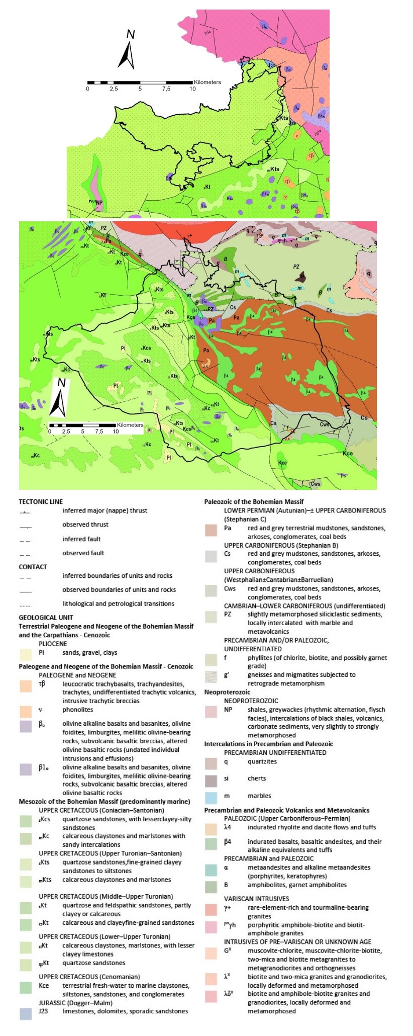
[17]	Uličný D (2001) Depositional systems and sequence stratigraphy of coarse-grained deltas in a shallow-marine, strike-slip setting: The Bohemian Cretaceous Basin, Czech Republic. Sedimentology 48: 599-628. doi: 10.1046/j.1365-3091.2001.00381.x
[18]	Czech geological service (2020) Geological map 1: 500000, Prague. Available from: https://mapy.geology.cz/geological_map500/?locale=en.
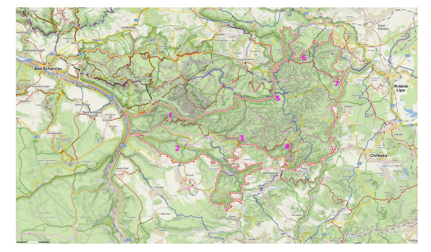
[19]	Czech Switzerland National Park (2020) Main Topics. Available from: https://www.npcs.cz/.
[20]	UNESCO Global Geopark Bohemian Paradise (2020) Global Geopark UNESCO Bohemian Paradise. Available from: http://www.geoparkceskyraj.cz/.
[21]	Czech Statistical Office (2020) Public Database. Available from: https://vdb.czso.cz/vdbvo2/faces/en/index.jsf.
[22]	Hastie T, Tibshirani R, Friedman J (2009) The Elements of Statistical Learning. 2^nd Ed. New York: Springer.
[23]	Butler RW (1980) The concept of tourism area cycle of evolution: implications for management of resources. Can Geogr 24: 5-12. doi: 10.1111/j.1541-0064.1980.tb00970.x
[24]	Butler RW (2009) Tourism in the future: Cycles, waves or wheels? Futures 41: 346-352. doi: 10.1016/j.futures.2008.11.002
[25]	Butler R, Wall G (1985) Introduction: Themes in research on the evolution of tourism. Ann Tour Res 12: 287-296. doi: 10.1016/0160-7383(85)90001-5
[26]	Drápela E, Bašta J (2018) Quantifying the power of border effect on Liberec region borders. Geogr Inf 22: 51-60.
[27]	Kubalíková L, Bajer A, Drápela E, et al. (2019) Cultural functions and services of geodiversity within urban areas (with a special regard on tourism and recreation). In: Fialova J (ed.), Public Recreation and Landscape Protection—With Sense Hand in Hand... Brno: Mendel Univ, 84-89.
[28]	Shekhar S, Kumar P, Chauhan G, et al. (2019) Conservation and Sustainable Development of Geoheritage, Geopark, and Geotourism: A Case Study of Cenozoic Successions of Western Kutch, India. Geoheritage 11: 1475-1488. doi: 10.1007/s12371-019-00362-5
[29]	Erikstad L (2013) Geoheritage and geodiversity management—the questions for tomorrow. Proc Geol Assoc 124: 713-719. doi: 10.1016/j.pgeola.2012.07.003
[30]	Eder W (2008) Geoparks—Promotion of Earth Sciences through Geoheritage Conservation, Education and Tourism. J Geol Soc India 72: 149-154.
[31]	Mariotto FP, Venturini C (2017) Strategies and Tools for Improving Earth Science Education and Popularization in Museums. Geoheritage 9: 187-194. doi: 10.1007/s12371-016-0194-z
[32]	Catana MM, Brilha JB (2020) The Role of UNESCO Global Geoparks in Promoting Geosciences Education for Sustainability. Geoheritage 12: 1. doi: 10.1007/s12371-020-00440-z

This article has been cited by:

1.	Erdal Karapinar, Andreea Fulga, Seher Sultan Yeşilkaya, Santosh Kumar, Fixed Points of Proinov Type Multivalued Mappings on Quasimetric Spaces, 2022, 2022, 2314-8888, 1, 10.1155/2022/7197541
2.	Mi Zhou, Xiaolan Liu, Naeem Saleem, Andreea Fulga, Nihal Özgür, A New Study on the Fixed Point Sets of Proinov-Type Contractions via Rational Forms, 2022, 14, 2073-8994, 93, 10.3390/sym14010093
3.	Salvador Romaguera, Basic Contractions of Suzuki-Type on Quasi-Metric Spaces and Fixed Point Results, 2022, 10, 2227-7390, 3931, 10.3390/math10213931
4.	Salvador Romaguera, On Protected Quasi-Metrics, 2024, 13, 2075-1680, 158, 10.3390/axioms13030158

Reader Comments

Your name:*

Email:*
© 2021 the Author(s), licensee AIMS Press. This is an open access article distributed under the terms of the Creative Commons Attribution License (http://creativecommons.org/licenses/by/4.0)