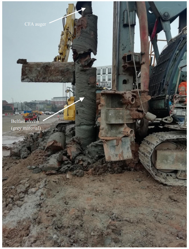
Belfast, the capital city of Northern Ireland and the second largest city on the island of Ireland, has experienced significant construction activity in recent years, yet relatively little has been published on the problematic soft estuarine deposits known locally as sleech which underlie the city and its hinterland. Results of a detailed characterization of the sleech at a site near Holywood, Co. Down, 8 km northeast of the city centre, are presented in this paper. This characterization was carried out in conjunction with a unique suite of full-scale foundation load tests at the site, commencing in the late 1990s. In situ tests clearly identified distinct sandy and silty horizons within the deposit, the bulk of which is a high-plasticity lightly-overconsolidated organic clayey silt, with clay content increasing with depth and clay fraction dominated by illite and chlorite. Both the moderate organic content and presence of diatom microfossils explain the relatively high Atterberg limits, the high compression index and the high friction angle of this material. Undrained shear strengths in triaxial compression fall at the upper end of the expected range based on a widely-used correlation with overconsolidation ratio, but are broadly compatible with in situ shear vane strengths corrected for plasticity index. The constant volume friction angle is remarkably insensitive to the specimen's stress history and the particle size distribution. Despite the high silt content, permeabilities and coefficients of consolidation are more typical of a clay than a silt. While the sleech behaviour is shown to be broadly similar to the estuarine deposits at the well-characterised geotechnical test bed at Bothkennar in Scotland, the paper illustrates that low OCR clays can have their own distinguishing characteristics.
Citation: Bryan A McCabe, Barry M Lehane. Geotechnical characteristics of Belfast's estuarine clayey silt (sleech)[J]. AIMS Geosciences, 2025, 11(1): 91-116. doi: 10.3934/geosci.2025006
Belfast, the capital city of Northern Ireland and the second largest city on the island of Ireland, has experienced significant construction activity in recent years, yet relatively little has been published on the problematic soft estuarine deposits known locally as sleech which underlie the city and its hinterland. Results of a detailed characterization of the sleech at a site near Holywood, Co. Down, 8 km northeast of the city centre, are presented in this paper. This characterization was carried out in conjunction with a unique suite of full-scale foundation load tests at the site, commencing in the late 1990s. In situ tests clearly identified distinct sandy and silty horizons within the deposit, the bulk of which is a high-plasticity lightly-overconsolidated organic clayey silt, with clay content increasing with depth and clay fraction dominated by illite and chlorite. Both the moderate organic content and presence of diatom microfossils explain the relatively high Atterberg limits, the high compression index and the high friction angle of this material. Undrained shear strengths in triaxial compression fall at the upper end of the expected range based on a widely-used correlation with overconsolidation ratio, but are broadly compatible with in situ shear vane strengths corrected for plasticity index. The constant volume friction angle is remarkably insensitive to the specimen's stress history and the particle size distribution. Despite the high silt content, permeabilities and coefficients of consolidation are more typical of a clay than a silt. While the sleech behaviour is shown to be broadly similar to the estuarine deposits at the well-characterised geotechnical test bed at Bothkennar in Scotland, the paper illustrates that low OCR clays can have their own distinguishing characteristics.

| [1] | Hancock M (2019) Ground improvement: slaying the sleech, Ground Engineering. Available from: https://www.geplus.co.uk/features/ground-improvement-slaying-sleech-20-11-2019/. |
| [2] | Crooks JHA (1973) Laboratory studies of the Belfast estuarine deposits. PhD thesis, Queens University Belfast. |
| [3] |
Crooks JHA, Graham J (1972) Stress-strain properties of Belfast estuarine clay. Eng Geol 6: 275–288. https://doi.org/10.1016/0013-7952(72)90012-9 doi: 10.1016/0013-7952(72)90012-9

|
| [4] |
Crooks JHA, Graham J (1976) Geotechnical properties of the Belfast estuarine deposits. Géotechnique 26: 293–315. https://doi.org/10.1680/geot.1976.26.2.293 doi: 10.1680/geot.1976.26.2.293
|
| [5] | Bell A (1977) Laboratory Studies of the Belfast Estuarine Deposits. PhD Thesis, Queen's University of Belfast. |
| [6] |
Gregory BJ, Bell AL (1991) Geotechnical properties of Quaternary deposits in the Belfast area. Geol Soc Eng Geol Spec Publ 7: 219–228. https://doi.org/10.1144/GSL.ENG.1991.007.01.20 doi: 10.1144/GSL.ENG.1991.007.01.20
|
| [7] | McCabe BA (2002) Experimental investigations of driven pile group behaviour in Belfast soft clay. PhD thesis, Trinity College Dublin. |
| [8] | Hight DW, Paul MA, Barras BF, et al. (2003) The characterization of Bothkennar Clay. Charact Eng Prop Nat Soils 1: 543–597. |
| [9] | Lehane BM, Jardine RJ, McCabe BA (2003) One-way axial cyclic tension loading of driven piles in clay. Proceedings of the BGA International Conference on Foundations, 493–506. |
| [10] | McCabe BA, Lehane BM (2003) Stress changes associated with driving pile groups in clayey silt. Proceedings of the 13th European Conference on Soil Mechanics and Geotechnical Engineering, National University of Ireland Galway, 2: 271–276. |
| [11] |
McCabe BA, Lehane BM (2006) Behavior of axially loaded pile groups driven in clayey silt. J Geotech Geoenviron Eng 132: 401–410. https://doi.org/10.1061/(ASCE)1090-0241(2006)132:3(401) doi: 10.1061/(ASCE)1090-0241(2006)132:3(401)
|
| [12] | McCabe BA, Lehane BM (2006) Prediction of pile group response using a simplified non-linear finite element model, Methods in Geotechnical Engineering, CRC Press, Graz, 589–594. |
| [13] | McCabe BA, Lehane BM (2008) Measured and predicted t-z curves for a driven single pile in lightly overconsolidated silt. Proceedings of the 3rd International Conference on Site Characterization, Taipei, 487–491. |
| [14] | McCabe BA, Phillips DT (2008) Design lessons from full-scale foundation load tests. Proceedings of the 3rd International Conference on Site Characterization, Taipei, 615–620. |
| [15] | McCabe BA, Gavin KG, Kennelly ME (2008) Installation of a reduced-scale pile group in silt. 2nd BGA International Conference on Foundations, IHS BRE Press, Dundee, 1: 607–616. |
| [16] | Doherty P (2010) Factors affecting the capacity of piles in clay. PhD thesis, University College Dublin. |
| [17] |
Gavin KG, Gallagher D, Doherty P, et al. (2010) Field investigation of the effect of installation method on the shaft resistance of piles in clay. Can Geotech J 47: 730–741. https://doi.org/10.1139/T09-146 doi: 10.1139/T09-146
|
| [18] |
Doherty P, Gavin KG (2013) Pile aging in cohesive soils. J Geotech Geoenviron Eng 139: 1620–1624. https://doi.org/10.1061/(ASCE)GT.1943-5606.0000884 doi: 10.1061/(ASCE)GT.1943-5606.0000884
|
| [19] |
McCabe BA, Sexton BG, Lehane BM (2013) Operational coefficient of consolidation around a pile group in clay/silt. Geotech Geol Eng 31: 183–197. https://doi.org/10.1007/s10706-012-9579-1 doi: 10.1007/s10706-012-9579-1
|
| [20] | Lehane BM, Phillips DT, Paul TS, et al. (1999) Instrumented piles subjected to combined vertical and lateral loads. Proceedings of the 12th European Conference on Soil Mechanics and Geotechnical Engineering, Amsterdam, 2: 1145–1150. |
| [21] | Phillips DT (2002) Field tests on single piles subjected to lateral and combined axial and lateral loads. PhD Thesis, Trinity College Dublin. |
| [22] |
Lehane BM (2003) Vertically loaded shallow foundation on soft clayey silt: A case history. Geotech Eng 156: 17–26. https://doi.org/10.1680/geng.2003.156.1.17 doi: 10.1680/geng.2003.156.1.17
|
| [23] | Timoney MJ (2015) Strength verification methods for stabilised soil-cement columns: a laboratory investigation of the PORT and PIRT. PhD thesis, University of Galway. |
| [24] |
Timoney MJ, McCabe BA (2017) Strength verification of stabilised soil-cement columns: a laboratory investigation of the Push-In Resistance Test (PIRT). Can Geotech J 54: 789–805. https://doi.org/10.1139/cgj-2016-0230 doi: 10.1139/cgj-2016-0230
|
| [25] |
Bowen DQ, Rose J, McCabe AM, et al. (1986) Correlation of Quaternary glaciations in England, Ireland, Scotland and Wales. Quat Sci Rev 5: 299–340. https://doi.org/10.1016/0277-3791(86)90194-0 doi: 10.1016/0277-3791(86)90194-0
|
| [26] | Wilson HE (1972) Recent Geology of Northern Ireland, HMSO, Belfast. |
| [27] | Manning PI, Robbie JA, Wilson HE (1970) Geology of Belfast and the Lagan Valley, HMSO, Belfast. |
| [28] |
Hight DW, Bond AJ, Legge JD (1992) Characterization of the Bothkennar clay: an overview. Géotechnique 42: 303–347. https://doi.org/10.1680/geot.1992.42.2.303 doi: 10.1680/geot.1992.42.2.303
|
| [29] | Mitchell JK (1976) Fundamentals of Soil Behaviour, 1st edition, London: Wiley. |
| [30] | Lutenegger AJ, Cerato A (2001) Surface area and engineering properties of fine-grained soils. Proceedings of the 15th International Conference on Soil Mechanics and Geotechnical Engineering, 1–3: 603–606. |
| [31] |
Xu S, Feng Q, Deng Y, et al. (2024) Effect of diatom inclusion on physical property identification of soft clay. J Soils Sediments 24: 603–614. https://doi.org/10.1007/s11368-023-03673-x doi: 10.1007/s11368-023-03673-x
|
| [32] |
Gundersen AS, Hansen RC, Lunne T, et al. (2019) Characterization and engineering properties of the NGTS Onsøy soft clay site. AIMS Geosci 5: 665–703. https://doi.org/10.3934/geosci.2019.3.665 doi: 10.3934/geosci.2019.3.665
|
| [33] | Shibuya S, Tamrakar SB, Thermast N (2001) Geotechnical site characterization on engineering properties of Bangkok Clay. J Southeast Asian Geotech Soc 32: 139–151. |
| [34] |
Low HE, Landon Maynard M, Randolph MF, et al. (2011) Geotechnical characterisation and engineering properties of Burswood clay. Géotechnique 61: 575–591. https://doi.org/10.1680/geot.9.P.035 doi: 10.1680/geot.9.P.035
|
| [35] |
Zhang X, Liu X, Xu Y, et al. (2024) Compressibility, permeability and microstructure of fine-grained soils containing diatom microfossils. Géotechnique 74: 661–675. https://doi.org/10.1680/jgeot.22.00155 doi: 10.1680/jgeot.22.00155
|
| [36] |
Robertson PK (1990) Soil classification using the cone penetration test. Can Geotech J 27: 151–158. https://doi.org/10.1139/t90-014 doi: 10.1139/t90-014
|
| [37] | Suzuki Y, Lehane BM (2014) Field observations of CPT penetration rate effects in Burswood clay. Proceedings of 3rd International Conference on Cone Penetration Testing, 403–410. |
| [38] | Long M, Colreavy C, Ward D, et al. (2014) Piezoball tests in soft Irish clays. Proceedings of the 3rd International Symposium on Cone Penetration Testing, Las Vegas, Nevada, 467–475. |
| [39] | Houlsby GT, Teh CI (1988) Analysis of the Piezocone in Clay. Conference on Penetration Testing, Balkema, Rotterdam, 777–783. |
| [40] |
Leroueil S, Lerat P, Hight DW, et al. (1992) Hydraulic Conductivity of a Recent Estuarine Silty Clay at Bothkennar, Scotland. Géotechnique 42: 275–288. https://doi.org/10.1680/geot.1992.42.2.275 doi: 10.1680/geot.1992.42.2.275
|
| [41] |
Shiwakoti DR, Tanaka H, Tanaka M, et al. (2002) Influences of diatom microfossils on engineering properties of soils. Soils Found 42: 1–17. https://doi.org/10.3208/sandf.42.3_1 doi: 10.3208/sandf.42.3_1
|
| [42] |
McCabe BA, Sheil BB, Buggy F, et al. (2014) Empirical correlations for the compression index of Irish soft soils. Proc Inst Civ Eng Geotech Eng 167: 510–517. https://doi.org/10.1680/geng.13.00116 doi: 10.1680/geng.13.00116
|
| [43] |
Burland JB, Eng F (1990) On the Compressibility and Shear Strength of Natural Clays. Géotechnique 40: 329–378. https://doi.org/10.1680/geot.1990.40.3.329 doi: 10.1680/geot.1990.40.3.329
|
| [44] |
Mesri G, Godlewski PM (1977) Time and stress-compressibility inter-relationship. J Geotech Eng Div 103: 417–430. https://doi.org/10.1061/AJGEB6.0000421 doi: 10.1061/AJGEB6.0000421
|
| [45] | Glossop NH, Saville DR, Moore JS, et al. (1979) Geotechnical aspects of shallow tunnel construction in Belfast estuarine deposits. Tunnelling 79, London, 45–56. |
| [46] |
DeGroot DJ, Landon ME, Poirier SE (2019) Geology and engineering properties of sensitive Boston Blue Clay at Newbury, Massachusetts. AIMS Geosci 5: 412–447. https://doi.org/10.3934/geosci.2019.3.412 doi: 10.3934/geosci.2019.3.412
|
| [47] | Chen C, Wang Y, Sun Z, et al. (2024) Rate effects of cylindrical cavity expansion in fine grained soil. J Rock Mech Geotech Eng, in press. https://doi.org/10.1016/j.jrmge.2024.09.032 |
| [48] |
Davies JA, Humpheson C (1981) Comparison between the performance of two types of vertical drain beneath a trial embankment in Belfast. Géotechnique 31: 19–31. https://doi.org/10.1680/geot.1981.31.1.19 doi: 10.1680/geot.1981.31.1.19
|
| [49] | Jaky J (1944) The coefficient of earth pressure at rest. J Soc Hung Archit Eng, 355–358. |
| [50] | Ladd CC, Foott R, Ishihara K, et al. (1977) Stress-Deformation and Strength Characteristics. Proceedings of the 9th International Conference on Soil Mechanics and Foundation Engineering, Tokyo, 2: 421–494. |
| [51] | Padfield CJ, Mair RJ (1983) Design of retaining walls embedded in soft clay, CIRIA report 104. |
| [52] |
Jardine RJ, Chow FC, Matsumoto T, et al. (1998) A new design procedure for driven piles and its applications to two Japanese clays. Soils Found 38: 207–219. https://doi.org/10.3208/sandf.38.207 doi: 10.3208/sandf.38.207
|
| [53] |
Lupini JF, Skinner AE, Vaughan PR (1981) Drained residual strength of cohesive soils. Géotechnique 31: 181–213. https://doi.org/10.1680/geot.1981.31.2.181 doi: 10.1680/geot.1981.31.2.181
|
| [54] | Strick van Linschoten CJ (2004) Driven pile capacity in organic clays with particular reference to square piles in Belfast sleech. MSc thesis, Imperial College London. |
| [55] |
Doherty P, Gavin KG (2009) Experimental investigation of the effect of shearing rate on the capacity of piles in soft silt. Contemp Top Deep Found, 575–582. https://doi.org/10.1061/41021(335)72 doi: 10.1061/41021(335)72
|


Figures(17) / Tables(2)

Bryan A McCabe, Barry M Lehane. Geotechnical characteristics of Belfast's estuarine clayey silt (sleech)[J]. AIMS Geosciences, 2025, 11(1): 91-116. doi: 10.3934/geosci.2025006


 DownLoad: