In this work, we analyzed simultaneous observations of solar particles and solar electromagnetic ultraviolet (UV) radiation during solar events from January 2024 to May 2024. Measurement campaigns to study the effects of space radiation on the terrestrial atmosphere were conducted in the framework of the project BIOSPHERE. We show the results of the campaign in Brussels from 1 January 2024 to 31 March 2024, during which several solar energetic particle (SEP) events were observed by the spacecraft GOES and OMNI, together with two big geomagnetic storms in March 2024 and May 2024 associated with solar eruptions. The last two events combine the arrival of a SEP event with a geomagnetic storm. On 11 May 2024, the biggest geomagnetic storm for the last 20 years was observed. These events enabled us to identify effects due to UV, solar particles, and geomagnetic storms. The impact of these events on the terrestrial radiation belts, illustrated by satellite observations like PROBA-V/EPT and on the atmospheric ozone using AURA/MLS is demonstrated. For the measurement campaign, muon and neutron monitors showed a Forbush decrease only during the geomagnetic storm at the end of March 2024 and in May 2024. Complemented by a simulation of radiation effects on the ionization rate of the atmosphere as a function of the altitude, the extensive range of different observations available during this measurement campaign demonstrated that SEP and geomagnetic storms due to solar eruptions had very different effects on the terrestrial atmosphere. The geomagnetic storms mainly modified the energetic electrons trapped in the space environment of the Earth and affected the ionization of the atmosphere above 60 km. They also modified the cosmic ray injections, mainly at high latitudes, creating Forbush decrease for the most intense ones. SEP events injected energetic protons in the atmosphere that could penetrate deeper in the atmosphere because they had more energy than the electrons. They could impact ozone, mainly at high altitude in the thermosphere. Solar activity variation associated with the rotation of the solar active regions in 27 days modulated UV. The measurements of these electromagnetic and particle radiations are crucial because they have important health implications.
Citation: Viviane Pierrard, David Bolsée, Alexandre Winant, Amer Al-Qaaod, Faton Krasniqi, Maximilien Péters de Bonhome, Edith Botek, Lionel Van Laeken, Danislav Sapundjiev, Roeland Van Malderen, Alexander Mangold, Iva Ambrozova, Marek Sommer, Jakub Slegl, Styliani A Geronikolou, Alexandros G Georgakilas, Alexander Dorn, Benjamin Rapp, Jaroslav Solc, Lukas Marek, Cristina Oancea, Lionel Doppler, Ronald Langer, Sarah Walsh, Marco Sabia, Marco Vuolo, Alex Papayannis, Carlos Granja. BIOSPHERE measurement campaign from January 2024 to March 2024 and in May 2024: Effects of the solar events on the radiation belts, UV radiation and ozone in the atmosphere[J]. AIMS Geosciences, 2025, 11(1): 117-154. doi: 10.3934/geosci.2025007
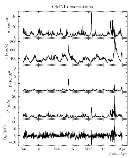
In this work, we analyzed simultaneous observations of solar particles and solar electromagnetic ultraviolet (UV) radiation during solar events from January 2024 to May 2024. Measurement campaigns to study the effects of space radiation on the terrestrial atmosphere were conducted in the framework of the project BIOSPHERE. We show the results of the campaign in Brussels from 1 January 2024 to 31 March 2024, during which several solar energetic particle (SEP) events were observed by the spacecraft GOES and OMNI, together with two big geomagnetic storms in March 2024 and May 2024 associated with solar eruptions. The last two events combine the arrival of a SEP event with a geomagnetic storm. On 11 May 2024, the biggest geomagnetic storm for the last 20 years was observed. These events enabled us to identify effects due to UV, solar particles, and geomagnetic storms. The impact of these events on the terrestrial radiation belts, illustrated by satellite observations like PROBA-V/EPT and on the atmospheric ozone using AURA/MLS is demonstrated. For the measurement campaign, muon and neutron monitors showed a Forbush decrease only during the geomagnetic storm at the end of March 2024 and in May 2024. Complemented by a simulation of radiation effects on the ionization rate of the atmosphere as a function of the altitude, the extensive range of different observations available during this measurement campaign demonstrated that SEP and geomagnetic storms due to solar eruptions had very different effects on the terrestrial atmosphere. The geomagnetic storms mainly modified the energetic electrons trapped in the space environment of the Earth and affected the ionization of the atmosphere above 60 km. They also modified the cosmic ray injections, mainly at high latitudes, creating Forbush decrease for the most intense ones. SEP events injected energetic protons in the atmosphere that could penetrate deeper in the atmosphere because they had more energy than the electrons. They could impact ozone, mainly at high altitude in the thermosphere. Solar activity variation associated with the rotation of the solar active regions in 27 days modulated UV. The measurements of these electromagnetic and particle radiations are crucial because they have important health implications.

| [1] |
Sinnhuber M, Nieder H, Wieters N (2012) Energetic Particle Precipitation and the Chemistry of the Mesosphere/Lower Thermosphere. Surv Geophys 33: 1281–1334. https://doi.org/10.1007/s10712-012-9201-3 doi: 10.1007/s10712-012-9201-3

|
| [2] | Krasniqi F (2023) Biosphere Newsletter, 1st issue. Available from: www.euramet-biosphere.eu. |
| [3] | Papayannis A, Gidarakou M, Mylonaki M, et al. (2023) Aerosol, Temperature and Water Vapor profiling during the BIOSPHERE Athens Campaign (June-August 2023). 4th European Lidar Conference, Cluj-Napoca, Romania. https://doi.org/10.5281/zenodo.10018507 |
| [4] |
Pierrard V, Lopez Rosson G, Borremans K, et al. (2014) The Energetic Particle Telescope: First results. Space Sci Rev 184: 87–106. https://doi.org/10.1007/s11214-014-0097-8 doi: 10.1007/s11214-014-0097-8
|
| [5] | Pierrard V (2024) Effects of the Sun on the space environment of the Earth, Presses Universitaires de Louvain, 208. https://i6doc.com/en/book/?gcoi = 28001100628290 |
| [6] | Evans D, Greer M (2000) Polar orbiting environmental satellite space environment monitor. NOAA National Geophysical Data Center. |
| [7] | Schwartz M, Froidevaux L, Livesey N, et al. (2020) MLS/Aura Level 2 Ozone (O3) Mixing Ratio V005, Greenbelt, MD, USA, Goddard Earth Sciences Data and Information Services Center (GES DISC). |
| [8] |
Smith AK, Espy PJ, Lopez-Puertas M, et al. (2018) Spatial and temporal structure of the tertiary ozone maximum in the polar winter mesosphere. J Geophys Res Atmos 123: 4373–4389. https://doi.org/10.1029/2017JD028030 doi: 10.1029/2017JD028030
|
| [9] | Winant A, Pierrard V, Botek E (2025) Ozone decrease observed in the upper atmosphere following the May 11th 2024 Mother's Day solar storm. Ann Geophys Discuss. [preprint]. https://doi.org/10.5194/angeo-2024-29 |
| [10] |
Banjac S, Herbst K, Heber B (2019) The atmospheric radiation interaction simulator (AtRIS): Description and validation. J Geophys Res Space Phys 124: 50–67. https://doi.org/10.1029/2018JA026042 doi: 10.1029/2018JA026042
|
| [11] |
Winant A, Pierrard V, Botek E, et al. (2023) The atmospheric influence on cosmic ray induced ionization and absorbed dose rates. Universe 9: 502. https://doi.org/10.3390/universe9120502 doi: 10.3390/universe9120502
|
| [12] |
Bilitza D, Pezzopane M, Truhlik V, et al. (2022) The International Reference Ionosphere model: A review and description of an ionospheric benchmark. Rev Geophys 60: e2022RG000792. https://doi.org/10.1029/2022RG000792 doi: 10.1029/2022RG000792
|
| [13] |
Pierrard V, Botek E, Darrouzet F (2021) Improving Predictions of the 3rd Dynamic Model of the Plasmasphere. Front Astron Space Sci 8: 681401. https://doi.org/10.3389/fspas.2021.681401 doi: 10.3389/fspas.2021.681401
|
| [14] |
Andersson ME, Verronen PT, Wang S, et al. (2012) Precipitating radiation belt electrons and enhancements of mesospheric hydroxyl during 2004–2009. J Geophys Res Atmos 117. https://doi.org/10.1029/2011JD017246 doi: 10.1029/2011JD017246
|
| [15] |
Wolff W, Dogan M, Luna H, et al. (2024) Absolute electron impact ionization cross-sections for CF4: Three dimensional recoil-ion imaging combined with the relative flow technique. Rev Sci Instrum 95: 095103. https://doi.org/10.1063/5.0219527 doi: 10.1063/5.0219527
|
| [16] |
Cyamukungu M, Benck S, Borisov S, et al. (2014) The Energetic Particle Telescope (EPT) on board PROBA-V: description of a new science-class instrument for particle detection in space. IEEE Trans Nucl Sci 61: 3667–3681. https://doi.org/10.1109/TNS.2014.2361955 doi: 10.1109/TNS.2014.2361955
|
| [17] |
McIlwain CE (1966) Magnetic coordinates. Space Sci Rev 5: 585–598. https://doi.org/10.1007/BF00167327 doi: 10.1007/BF00167327
|
| [18] |
Pierrard V, Botek E, Ripoll JF, et al. (2020) Electron dropout events and flux enhancements associated with geomagnetic storms observed by PROBA-V/EPT from 2013 to 2019. J Geophys Res Space Phys 125: e2020JA028487. https://doi.org/10.1029/2020JA028487 doi: 10.1029/2020JA028487
|
| [19] |
Pierrard V, Lopez Rosson G (2016) The effects of the big storm events in the first half of 2015 on the radiation belts observed by EPT/PROBA-V. Ann Geophys 34: 75–84. https://doi.org/10.5194/angeo-34-75-2016 doi: 10.5194/angeo-34-75-2016
|
| [20] |
Pierrard V, Ripoll J-F, Cunningham G, et al. (2021) Observations and simulations of dropout events and flux enhancements in October 2013: Comparing MEO equatorial with LEO polar orbit. J Geophys Res Space Phys 126: e2020JA028850. https://doi.org/10.1029/2020JA028850 doi: 10.1029/2020JA028850
|
| [21] |
Pierrard V, Botek E, Ripoll J-F, et al. (2021) Links of the plasmapause with other boundary layers of the magnetosphere: ionospheric convection, radiation belts boundaries, auroral oval. Front Astron Space Sci 8. https://doi.org/10.3389/fspas.2021.728531 doi: 10.3389/fspas.2021.728531
|
| [22] |
Cunningham GS, Botek E, Pierrard V, et al. (2020) Observation of High-Energy Electrons Precipitated by NWC Transmitter from PROBA-V Low-Earth Orbit Satellite. Geophys Res Lett 47: e2020GL089077. https://doi.org/10.1029/2020GL089077 doi: 10.1029/2020GL089077
|
| [23] |
Botek E, Pierrard V, Winant A (2023) Prediction of radiation belts electron fluxes at a Low Earth Orbit using neural networks with PROBA-V/EPT data. Space Weather 21: e2023SW003466. https://doi.org/10.1029/2023SW003466 doi: 10.1029/2023SW003466
|
| [24] |
Girgis KM, Hada T, Yoshikawa A, et al. (2023) Geomagnetic Storm Effects on the LEO Proton Flux during Solar Energetic Particle Events. Space Weather 21: e2023SW003664. https://doi.org/10.1029/2023SW003664 doi: 10.1029/2023SW003664
|
| [25] |
Pierrard V, Benck S, Botek E, et al. (2023) Proton flux variations during Solar Energetic Particle Events, minimum and maximum solar activity and splitting of the proton belt in the South Atlantic Anomaly. J Geophys Res Space Phys 128: e2022JA031202. https://doi.org/10.1029/2022JA031202 doi: 10.1029/2022JA031202
|
| [26] |
Pierrard V, Winant A, Botek E, et al. (2024) The Mother's Day solar storm of 11 May 2024 and its effect on Earth's radiation belts. Universe 10: 391. https://doi.org/10.3390/universe10100391 doi: 10.3390/universe10100391
|
| [27] |
Poikela T, Plosila J, Westerlund T, et al. (2014) Timepix3: a 65K channel hybrid pixel readout chip with simultaneous ToA/ToT and sparse readout. J Instrum 9: C05013. https://doi.org/10.1088/1748-0221/9/05/C05013 doi: 10.1088/1748-0221/9/05/C05013
|
| [28] |
Freiherr von Forstner JL, Dumbović M, Möstl C, et al. (2021) Radial evolution of the April 2020 stealth coronal mass ejection between 0.8 and 1 AU. Comparison of Forbush decreases at Solar Orbiter and near the Earth. Astron Astrophys 656. https://doi.org/10.1051/0004-6361/202039848 doi: 10.1051/0004-6361/202039848
|
| [29] | Krasniqi F, Stolzenberg U, Luchkov M, et al. (2022) PTB metrological infrastructure for the environmental dose assessment. PTB-Mitt 132: 21–31. |
| [30] |
Chilingarian A, Hovsepyan G, Arakelyan K, et al. (2009) Space environmental viewing and analysis network (SEVAN). Earth Moon Planets 104: 195. https://doi.org/10.1007/s11038-008-9288-1 doi: 10.1007/s11038-008-9288-1
|
| [31] |
Chilingarian A, Babayan V, Karapetyan T, et al. (2018) The SEVAN Worldwide network of particle detectors: 10 years of operation. Adv Space Res 61: 2680–2696. https://doi.org/10.1016/j.asr.2018.02.030 doi: 10.1016/j.asr.2018.02.030
|
| [32] |
Granja C, Jakubek J, Soukup P, et al. (2022) Spectral tracking of energetic charged particles in wide field-of-view with miniaturized telescope MiniPIX Timepix3 1 × 2 Stack. J Instrum 17: C03028. https://doi.org/10.1088/1748-0221/17/03/C03028 doi: 10.1088/1748-0221/17/03/C03028
|
| [33] |
Granja C, Pospisil S (2014) Quantum Dosimetry and Online Visualization of X-ray and Charged Particle Radiation in Aircraft at Operational Flight Altitudes with the Pixel Detector Timepix. Adv Space Res 54: 241–251. https://doi.org/10.1016/j.asr.2014.04.006 doi: 10.1016/j.asr.2014.04.006
|
| [34] |
Spogli L, Alberti T, Bagiacchi P, et al. (2024) The effects of the May 2024 Mother's Day superstorm over the Mediterranean sector: from data to public communication. Ann Geophys 67: PA218. https://doi.org/10.4401/ag-9117 doi: 10.4401/ag-9117
|
| [35] |
Themens DR, Elvidge S, McCaffrey A, et al. (2024) The high latitude ionospheric response to the major May 2024 geomagnetic storm: A synoptic view. Geophys Res Lett 51: e2024GL111677. https://doi.org/10.1029/2024GL111677 doi: 10.1029/2024GL111677
|
| [36] |
Pierrard V, Verhulst TGW, Chevalier J-M, et al. (2025) Effects of the geomagnetic superstorms of 10–11 May 2024 and 7–11 October 2024 on the ionosphere and plasmasphere. Atmosphere 16: 299. https://doi.org/10.3390/atmos16030299 doi: 10.3390/atmos16030299
|
| [37] |
Liu X, Xu J, Yue J, et al. (2025) Mesosphere and lower thermosphere temperature responses to the May 2024 Mother's Day storm. Geophys Res Lett 52: e2024GL112179. https://doi.org/10.1029/2024GL112179 doi: 10.1029/2024GL112179
|
| [38] |
Richard E, Harber D, Coddington O, et al. (2020) SI-traceable spectral irradiance radiometric characterization and absolute calibration of the TSIS-1 spectral irradiance monitor (SIM). Remote Sens 12: 1818. https://doi.org/10.3390/rs12111818 doi: 10.3390/rs12111818
|
| [39] |
DeLand MT, Cebula RP (1993) Composite MgII solar activity index for solar cycles 21 and 22. J Geophys Res Atmos 98: 12809–12823. https://doi.org/10.1029/93JD00421 doi: 10.1029/93JD00421
|
| [40] | Bossay S (2015) Impact de la variabilité solaire sur l'ozone de la moyenne atmosphère. PhD Thesis, Université Versailles Saint Quentin en Yvelines, France. https://theses.hal.science/tel-01139519/ |
| [41] |
De Bock V, De Backer H, Van Malderen R, et al. (2014) Relations between erythemal UV dose, global solar radiation, total ozone column and aerosol optical depth at Uccle, Belgium. Atmos Chem Phys 14: 12251–12270. https://doi.org/10.5194/acp-14-12251-2014 doi: 10.5194/acp-14-12251-2014
|
| [42] |
Rimmer JS, Redondas A, Karppinen T (2018) EuBrewNet—A European Brewer network (COST Action ES1207), an overview. Atmos Chem Phys 18: 10347–10353. https://doi.org/10.5194/acp-18-10347-2018 doi: 10.5194/acp-18-10347-2018
|
| [43] | McKinlay AF, Diffey BL (1987) A Reference Action Spectrum for Ultraviolet Induced Erythema in Human Skin. CIE J 6: 17–22. International Organization for Standardization and International Commission on Illumination. Erythema reference action spectrum and standard erythema dose (ISO/CIE 17166: 2019). Available from: https://www.iso.org. |
| [44] |
Geronikolou S, Zimeras S, Tsitomeneas S, et al. (2023) Total Solar Irradiance and Stroke Mortality by Neural Networks Modelling. Atmosphere 14: 114. https://doi.org/10.3390/atmos14010114 doi: 10.3390/atmos14010114
|
| [45] |
Zhai T, Zilli Vieira CL, Vokonas P, et al. (2024) Annual space weather fluctuations and telomere length dynamics in a longitudinal cohort of older men: the Normative Aging Study. J Expo Sci Environ Epidemiol 34: 1072–1080. https://doi.org/10.1038/s41370-023-00616-z doi: 10.1038/s41370-023-00616-z
|
| [46] |
Vencloviene J, Babarskiene RM, Kiznys D (2017) A possible association between space weather conditions and the risk of acute coronary syndrome in patients with diabetes and the metabolic syndrome. Int J Biometeorol 61: 159–167. https://doi.org/10.1007/s00484-016-1200-5 doi: 10.1007/s00484-016-1200-5
|
| [47] |
Zilli Vieira CL, Chen K, Garshick E, et al. (2022) Geomagnetic disturbances reduce heart rate variability in the Normative Aging Study. Sci Total Environ 839: 156235. https://doi.org/10.1016/j.scitotenv.2022.156235 doi: 10.1016/j.scitotenv.2022.156235
|
| [48] | Halberg F, Cornélissen G, Katinas G, et al. (2007) Chronomics and Genetics. Scr Med (Brno) 80: 133–150. |
| [49] | Halberg F, Cornélissen G, Katinas GS, et al. (2010) Cosmic Inheritance Rules: Implications for Health Care and Science. Scr Med (Brno) 83: 5–15 |
| [50] |
Geronikolou S, Leontitsis A, Petropoulos V, et al. (2020) Cyclic stroke mortality variations follow sunspot patterns. F1000Research 9: 1088. https://doi.org/10.12688/f1000research.24794.2 doi: 10.12688/f1000research.24794.2
|
| [51] |
Persinger MA (1997) Geomagnetic variables and behavior: LXXXIII. Increased geomagnetic activity and group aggression in chronic limbic epileptic male rats. Percept Motor Skill 85(3_suppl): 1376–1378. https://doi.org/10.2466/pms.1997.85.3f.1376 doi: 10.2466/pms.1997.85.3f.1376
|
| [52] | Halberg F, Siutkina EV, Cornelissen G (1998) Chronomes render predictable the otherwise-neglected human "physiological range": position paper of the BIOCOS project, BIOsphere and the COSmos. Fiziologiia Chel 24: 14–21. |
| [53] |
Mulligan B, Koren S (2021) Geopsychology of instrumental aggression: daily concurrence of global terrorism and solar-geomagnetic activity (1970–2018). Adv Soc Sci Res J 8: 487–499. https://doi.org/10.14738/assrj.85.10266 doi: 10.14738/assrj.85.10266
|
| [54] | Geronikolou S, Petropoulos V (2005) Stratospheric ozone, density variation solar activity and biological phenomena. HELLASET International Congress Cephalonia. |
| [55] | Geronikolou SA (2014) Evaluation of chronomes in the Greek population and their relation to solar and atmospheric activity cycles, The Mediterranean City 2014 Proceedings, Mariolopoulos-Kanaginis Foundation, 16–17. |
| [56] |
Stoupel E (2015) Considering space weather forces interaction on human health: the equilibrium paradigm in clinical cosmobiology—is it equal? J Basic Clin Physiol Pharmacol 26: 147–151. https://doi.org/10.1515/jbcpp-2014-0059 doi: 10.1515/jbcpp-2014-0059
|
| [57] |
Davis GE, Lowell WE (2006) Solar cycles and their relationship to human disease and adaptability. Med Hypotheses 67: 447–461. https://doi.org/10.1016/j.mehy.2006.03.011 doi: 10.1016/j.mehy.2006.03.011
|
| [58] |
Papathanasopoulos P, Preka-Papadema P, Gkotsinas A, et al. (2016) The possible effects of the solar and geomagnetic activity on multiple sclerosis. Clin Neurol Neurosurg 146: 82–89. https://doi.org/10.1016/j.clineuro.2016.04.023 doi: 10.1016/j.clineuro.2016.04.023
|
| [59] | Halberg F, Cornélissen G, Otsuka K, et al. (2000) Cross-spectrally coherent ~10.5- and 21-year biological and physical cycles, magnetic storms and myocardial infarctions. Neuro Endocrinol Lett 21: 233–258. |
| [60] | Samsonov SN, Manykina VI, Kleimenova NG, et al. (2016) The HELIO-geophysical storminess health effects in the cardio-vascular system of a human in the middle and high latitudes. Wiad Lek 69(3 pt 2): 537–541. |
| [61] |
Zilli Vieira CL, Alvares D, Blomberg A, et al. (2019) Geomagnetic disturbances driven by solar activity enhance total and cardiovascular mortality risk in 263 U.S. cities. Environ Health 18: 83. https://doi.org/10.1186/s12940-019-0516-0 doi: 10.1186/s12940-019-0516-0
|
| [62] |
Geronikolou SA, Pavlopoulou A, Kanaka-Gantenbein C, et al. (2018) Inter-species functional interactome of nuclear steroid receptors (R1). Front Biosci (Elite Ed) 10: 208–228. https://doi.org/10.2741/e818 doi: 10.2741/e818
|


Figures(21) / Tables(1)

Viviane Pierrard, David Bolsée, Alexandre Winant, Amer Al-Qaaod, Faton Krasniqi, Maximilien Péters de Bonhome, Edith Botek, Lionel Van Laeken, Danislav Sapundjiev, Roeland Van Malderen, Alexander Mangold, Iva Ambrozova, Marek Sommer, Jakub Slegl, Styliani A Geronikolou, Alexandros G Georgakilas, Alexander Dorn, Benjamin Rapp, Jaroslav Solc, Lukas Marek, Cristina Oancea, Lionel Doppler, Ronald Langer, Sarah Walsh, Marco Sabia, Marco Vuolo, Alex Papayannis, Carlos Granja. BIOSPHERE measurement campaign from January 2024 to March 2024 and in May 2024: Effects of the solar events on the radiation belts, UV radiation and ozone in the atmosphere[J]. AIMS Geosciences, 2025, 11(1): 117-154. doi: 10.3934/geosci.2025007


 DownLoad: