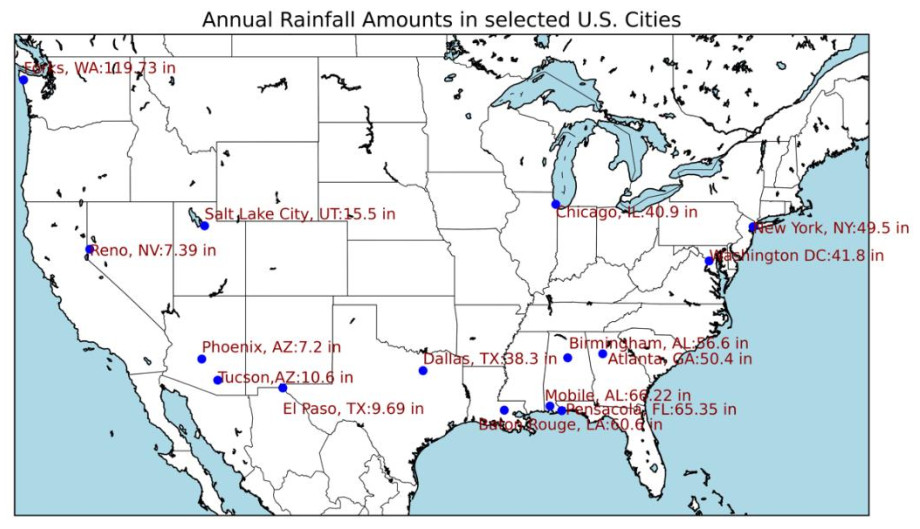
With the increasing impacts of climate change, there is a growing demand for accessible tools that can provide reliable future climate information to support planning, finance, and other decision-making applications. Large language models (LLMs), such as GPT-4o, present a promising approach to bridging the gap between complex climate data and the general public, offering a way for non-specialist users to obtain essential climate insights through natural language interaction. However, an essential challenge remains underexplored: Evaluating the ability of LLMs to provide accurate and reliable future climate predictions, which is crucial for applications that rely on anticipating climate trends. In this study, we investigated the capability of GPT-4o in predicting rainfall at short-term (15-day) and long-term (12-month) scales. We designed a series of experiments to assess GPT's performance under different conditions, including scenarios with and without expert data inputs. Our results indicated that GPT, when operating independently, tended to generate conservative forecasts, often reverting to historical averages in the absence of clear trend signals. This study highlights the potential and challenges of applying LLMs for future climate predictions, providing insights into their integration with climate-related applications and indicating directions for enhancing their predictive capabilities in the field.
Citation: Yang Wang, Hassan A. Karimi. Exploring large language models for climate forecasting[J]. Applied Computing and Intelligence, 2025, 5(1): 1-13. doi: 10.3934/aci.2025001
With the increasing impacts of climate change, there is a growing demand for accessible tools that can provide reliable future climate information to support planning, finance, and other decision-making applications. Large language models (LLMs), such as GPT-4o, present a promising approach to bridging the gap between complex climate data and the general public, offering a way for non-specialist users to obtain essential climate insights through natural language interaction. However, an essential challenge remains underexplored: Evaluating the ability of LLMs to provide accurate and reliable future climate predictions, which is crucial for applications that rely on anticipating climate trends. In this study, we investigated the capability of GPT-4o in predicting rainfall at short-term (15-day) and long-term (12-month) scales. We designed a series of experiments to assess GPT's performance under different conditions, including scenarios with and without expert data inputs. Our results indicated that GPT, when operating independently, tended to generate conservative forecasts, often reverting to historical averages in the absence of clear trend signals. This study highlights the potential and challenges of applying LLMs for future climate predictions, providing insights into their integration with climate-related applications and indicating directions for enhancing their predictive capabilities in the field.

| [1] |
S. D. Campbell, F. X. Diebold, Weather forecasting for weather derivatives, J. Am. Stat. Assoc., 100 (2005), 6–16. https://doi.org/10.1198/016214504000001051 doi: 10.1198/016214504000001051

|
| [2] |
C. Hewitt, S. Mason, D. Walland, The global framework for climate services, Nature Clim. Change, 2 (2012), 831–832. https://doi.org/10.1038/nclimate1745 doi: 10.1038/nclimate1745
|
| [3] | OpenAI, J. Achiam, S. Adler, S. Agarwal, L. Ahmad, I. Akkaya, et al., GPT-4 technical report, arXiv: 2303.08774. https://doi.org/10.48550/arXiv.2303.08774 |
| [4] |
J. K. Kim, M. Chua, M. Rickard, A. Lorenzo, ChatGPT and large language model (LLM) chatbots: the current state of acceptability and a proposal for guidelines on utilization in academic medicine, J. Pediatr. Urol., 19 (2023), 598–604. https://doi.org/10.1016/j.jpurol.2023.05.018 doi: 10.1016/j.jpurol.2023.05.018
|
| [5] |
M. Leippold, Thus spoke GPT-3: interviewing a large-language model on climate finance, Financ. Res. Lett., 53 (2023), 103617. https://doi.org/10.1016/j.frl.2022.103617 doi: 10.1016/j.frl.2022.103617
|
| [6] |
A. J. Thirunavukarasu, D. S. J. Ting, K. Elangovan, L. Gutierrez, T. F. Tan, D. S. W. Ting, Large language models in medicine, Nat. Med., 29 (2023), 1930–1940. https://doi.org/10.1038/s41591-023-02448-8 doi: 10.1038/s41591-023-02448-8
|
| [7] | H. Zhu, P. Tiwari, Climate change from large language models, arXiv: 2312.11985. https://doi.org/10.48550/arXiv.2312.11985 |
| [8] | M. Kraus, J. Bingler, M. Leippold, T. Schimanski, C. Senni, D. Stammbach, et al., Enhancing large language models with climate resources, arXiv: 2304.00116. https://doi.org/10.48550/arXiv.2304.00116 |
| [9] |
N. Koldunov, T. Jung, Local climate services for all, courtesy of large language models, Commun. Earth Environ., 5 (2024), 13. https://doi.org/10.1038/s43247-023-01199-1 doi: 10.1038/s43247-023-01199-1
|
| [10] | D. Thulke, Y. Gao, P. Pelser, R. Brune, R. Jalota, F. Fok, et al., Climategpt: towards AI synthesizing interdisciplinary research on climate change, arXiv: 2401.09646. https://doi.org/10.48550/arXiv.2401.09646 |
| [11] | N. Webersinke, M. Kraus, J. A. Bingler, M. Leippold, Climatebert: a pretrained language model for climate-related text, arXiv: 2110.12010. https://doi.org/10.48550/arXiv.2110.12010 |
| [12] | H. Nguyen, V. Nguyen, S. López-Fierro, S. Ludovise, R. Santagata, Simulating climate change discussion with large language models: considerations for science communication at scale, Proceedings of the 11th ACM Conference on Learning @ Scale, 2024, 28–38. https://doi.org/10.1145/3657604.3662033 |
| [13] | S. E. Brownell, J. V Price, L. Steinman, Science communication to the general public: why we need to teach undergraduate and graduate students this skill as part of their formal scientific training, J. Undergrad. Neurosci. Educ., 12 (2013), E6–E10. |
| [14] |
A. Sherstinsky, Fundamentals of recurrent neural network (RNN) and long short-term memory (LSTM) network, Physica D, 404 (2020), 132306. https://doi.org/10.1016/j.physd.2019.132306 doi: 10.1016/j.physd.2019.132306
|
| [15] |
Y. Wang, H. A. Karimi, Impact of spatial distribution information of rainfall in runoff simulation using deep learning method, Hydrol. Earth Syst. Sci., 26 (2022), 2387–2403. https://doi.org/10.5194/hess-26-2387-2022 doi: 10.5194/hess-26-2387-2022
|
| [16] |
M. Zhang, J. D. Rojo-Hernández, L. Yan, Ó. J. Mesa, U. Lall, Hidden tropical pacific sea surface temperature states reveal global predictability for monthly precipitation for sub-season to annual scales, Geophys. Res. Lett., 49 (2022), e2022GL099572. https://doi.org/10.1029/2022GL099572 doi: 10.1029/2022GL099572
|
| [17] |
R. Krishnan, M. Sugi, Pacific decadal oscillation and variability of the Indian summer monsoon rainfall, Clim. Dynam., 21 (2003), 233–242. https://doi.org/10.1007/s00382-003-0330-8 doi: 10.1007/s00382-003-0330-8
|
| [18] |
R. M. Trigo, J. L. Zêzere, M. L. Rodrigues, I. F. Trigo, The influence of the north atlantic oscillation on rainfall triggering of landslides near Lisbon, Nat. Hazards, 36 (2005), 331–354. https://doi.org/10.1007/s11069-005-1709-0 doi: 10.1007/s11069-005-1709-0
|
| [19] |
S. McGregor, C. Cassou, Y. Kosaka, A. S. Phillips, Projected ENSO teleconnection changes in CMIP6, Geophys. Res. Lett., 49 (2022), e2021GL097511. https://doi.org/10.1029/2021GL097511 doi: 10.1029/2021GL097511
|
| [20] |
K. M. Lau, H. Weng, Recurrent teleconnection patterns linking summertime precipitation variability over East Asia and North America, J. Meteorol. Soc. Japan, 80 (2002), 1309–1324. https://doi.org/10.2151/jmsj.80.1309 doi: 10.2151/jmsj.80.1309
|
| [21] |
S. Y. Wang, L. E. Hipps, R. R. Gillies, X. Jiang, A. L. Moller, Circumglobal teleconnection and early summer rainfall in the US Intermountain West, Theor. Appl. Climatol., 102 (2010), 245–252. https://doi.org/10.1007/s00704-010-0260-4 doi: 10.1007/s00704-010-0260-4
|
| [22] |
J. Wen, C. Wan, Q. Ye, J. Yan, W. Li, Disaster risk reduction, climate change adaptation and their linkages with sustainable development over the past 30 years: a review, Int. J. Disaster Risk Sci., 14 (2023), 1–13. https://doi.org/10.1007/s13753-023-00472-3 doi: 10.1007/s13753-023-00472-3
|
| [23] | Q. Wu, G. Bansal, J. Zhang, Y. Wu, B. Li, E. Zhu, et al., Autogen: enabling next-gen llm applications via multi-agent conversation framework, arXiv: 2308.08155. https://doi.org/10.48550/arXiv.2308.08155 |
| [24] |
Y. Lai, D. A. Dzombak, Use of historical data to assess regional climate change, J. Climate, 32 (2019), 4299–4320. https://doi.org/10.1175/JCLI-D-18-0630.1 doi: 10.1175/JCLI-D-18-0630.1
|


Figures(7)
Yang Wang, Hassan A. Karimi. Exploring large language models for climate forecasting[J]. Applied Computing and Intelligence, 2025, 5(1): 1-13. doi: 10.3934/aci.2025001


 DownLoad: