The extremophile microorganism Thermus scotoductus primarily exhibits aerobic metabolism, though some strains are capable of anaerobic growth, utilizing diverse electron acceptors. We focused on the T. scotoductus K1 strain, exploring its aerobic growth and metabolism, responses to various carbon sources, and characterization of its bioenergetic and physiological properties. The strain grew on different carbon sources, depending on their concentration and the medium's pH, demonstrating adaptability to acidic environments (pH 6.0). It was shown that 4 g L−1 glucose inhibited the specific growth rate by approximately 4.8-fold and 5.6-fold compared to 1 g L−1 glucose at pH 8.5 and pH 6.0, respectively. However, this inhibition was not observed in the presence of fructose, galactose, lactose, and starch. Extracellular and intracellular pH variations were mainly alkalifying during growth. At pH 6.0, the membrane potential (ΔΨ) was lower for all carbon sources compared to pH 8.5. The proton motive force (Δp) was lower only during growth on lactose due to the difference in the transmembrane proton gradient (ΔpH). Moreover, at pH 6.0 during growth on lactose, a positive Δp was detected, indicating the cells' ability to employ a unique energy-conserving strategy. Taken together, these findings concluded that Thermus scotoductus K1 exhibits different growth and bioenergetic properties depending on the carbon source, which can be useful for biotechnological applications. These findings offer valuable insights into how bacterial cells function under high-temperature conditions, which is essential for applying bioenergetics knowledge in future biotechnological advancements.
Citation: Hripsime Petrosyan, Karen Trchounian. Growth characteristics, redox potential changes and proton motive force generation in Thermus scotoductus K1 during growth on various carbon sources[J]. AIMS Microbiology, 2024, 10(4): 1052-1067. doi: 10.3934/microbiol.2024045
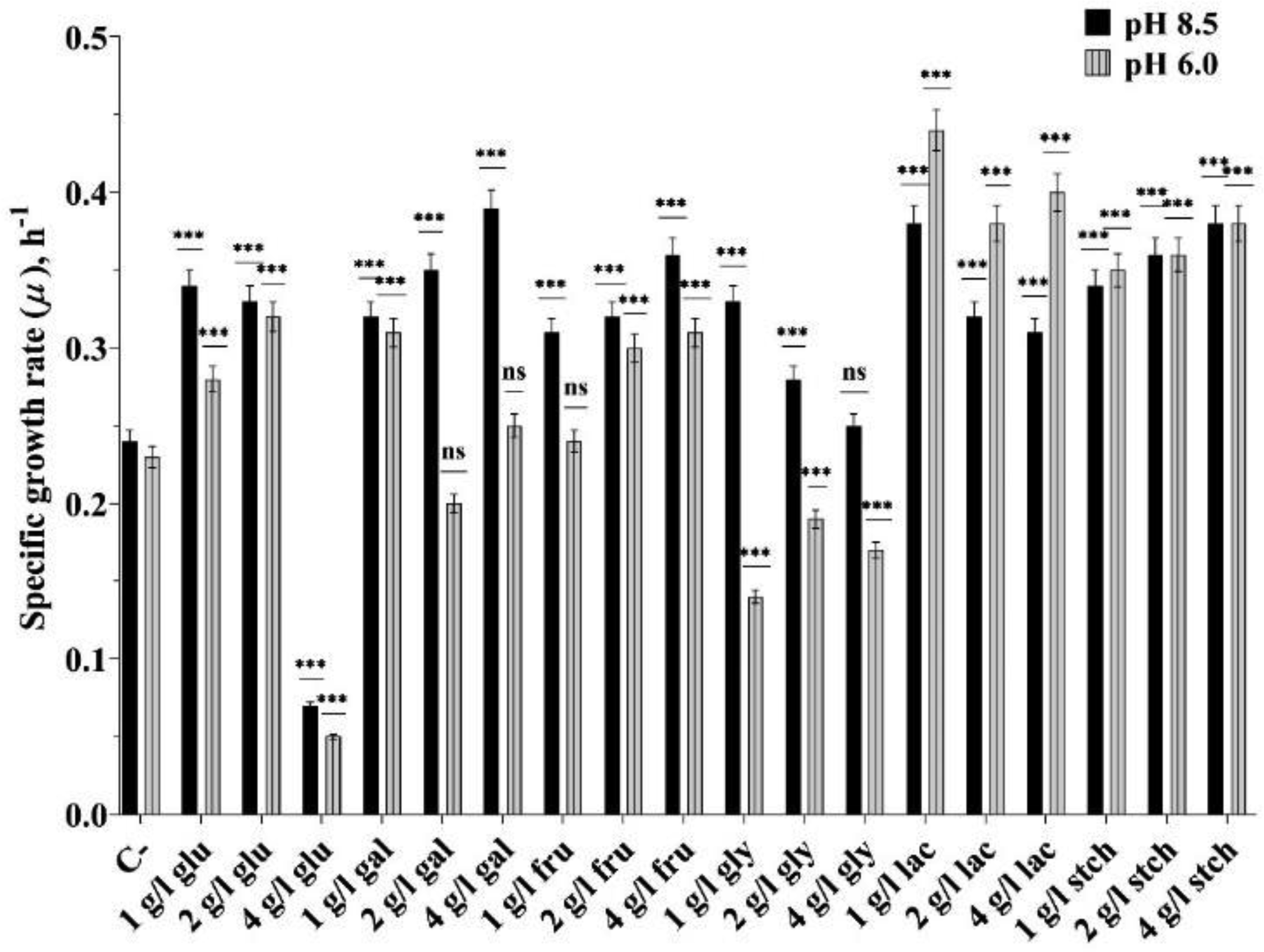
The extremophile microorganism Thermus scotoductus primarily exhibits aerobic metabolism, though some strains are capable of anaerobic growth, utilizing diverse electron acceptors. We focused on the T. scotoductus K1 strain, exploring its aerobic growth and metabolism, responses to various carbon sources, and characterization of its bioenergetic and physiological properties. The strain grew on different carbon sources, depending on their concentration and the medium's pH, demonstrating adaptability to acidic environments (pH 6.0). It was shown that 4 g L−1 glucose inhibited the specific growth rate by approximately 4.8-fold and 5.6-fold compared to 1 g L−1 glucose at pH 8.5 and pH 6.0, respectively. However, this inhibition was not observed in the presence of fructose, galactose, lactose, and starch. Extracellular and intracellular pH variations were mainly alkalifying during growth. At pH 6.0, the membrane potential (ΔΨ) was lower for all carbon sources compared to pH 8.5. The proton motive force (Δp) was lower only during growth on lactose due to the difference in the transmembrane proton gradient (ΔpH). Moreover, at pH 6.0 during growth on lactose, a positive Δp was detected, indicating the cells' ability to employ a unique energy-conserving strategy. Taken together, these findings concluded that Thermus scotoductus K1 exhibits different growth and bioenergetic properties depending on the carbon source, which can be useful for biotechnological applications. These findings offer valuable insights into how bacterial cells function under high-temperature conditions, which is essential for applying bioenergetics knowledge in future biotechnological advancements.

| [1] |
Sharp R, Williams R (1995) Thermus Species. New York: Springer. https://doi.org/10.1007/978-1-4615-1831-0 
|
| [2] |
Saghatelyan A, Panosyan H, Trchounian A, et al. (2021) Characteristics of DNA polymerase I from an extreme thermophile, Thermus scotoductus strain K1. MicrobiologyOpen 10: e1149. https://doi.org/10.1002/mbo3.1149
|
| [3] |
Kristjánsson JK, Hjörleifsdóttir S, Marteinsson VT, et al. (1994) Thermus scotoductus, sp. nov., a pigment-producing thermophilic bacterium from hot tap water in iceland and including Thermus sp. X-1. Syst Appl Microbiol 17: 44-50. https://doi.org/10.1016/S0723-2020(11)80030-5
|
| [4] |
Babák L, Šupinová P, Burdychová R (2013) Growth models of Thermus aquaticus and Thermus scotoductus. Acta Univ Agric Silvic Mendel Brun 60: 19-26. https://doi.org/10.11118/actaun201260050019
|
| [5] |
Aulitto M, Fusco S, Fiorentino G, et al. (2017) Thermus thermophilus as source of thermozymes for biotechnological applications: Homologous expression and biochemical characterization of an α-galactosidase. Microb Cell Fact 16: 28. https://doi.org/10.1186/s12934-017-0638-4
|
| [6] |
Wheaton S, Hauer M (2011) Recent applications of THERMUS. Phys Part Nuclei Lett 8: 869-873. https://doi.org/10.1134/S1547477111080152
|
| [7] |
Da Costa MS, Rainey FA, Nobre MF (2006) The Genus Thermus and relatives. The Prokaryotes . New York: Springer 797-812. https://doi.org/10.1007/0-387-30747-8_32
|
| [8] |
Elleuche S, Schröder C, Sahm K, et al. (2014) Extremozymes—biocatalysts with unique properties from extremophilic microorganisms. Curr Opin Biotechnol 29: 116-123. https://doi.org/10.1016/j.copbio.2014.04.003
|
| [9] | Chen L, Biosketch S, Sharmili A, et al. (2019) Advances and Trends in Biotechnology and Genetics, Vol. 3. London: Book Publisher International, SCIENCEDOMAIN International Ltd. http://dx.doi.org/10.9734/bpi/atbg/v3 |
| [10] |
Albers SV, Vossenberg JL, Driessen AJ, et al. (2001) Bioenergetics and solute uptake under extreme conditions. Extremophiles 5: 285-294. https://doi.org/10.1007/s007920100214
|
| [11] |
Somayaji A, Dhanjal CR, Lingamsetty R, et al. (2022) An insight into the mechanisms of homeostasis in extremophiles. Microbiol Res 263: 127115. https://doi.org/10.1016/j.micres.2022.127115
|
| [12] |
Vieille C, Zeikus GJ (2001) Hyperthermophilic Enzymes: Sources, uses, and molecular mechanisms for thermostability. Microbiol Mol Biol Rev 65: 1-43. https://doi.org/10.1128/MMBR.65.1.1-43.2001
|
| [13] |
Rekadwad BN, Li WJ, Gonzalez JM, et al. (2023) Extremophiles: the species that evolve and survive under hostile conditions. 3 Biotech 13: 316. https://doi.org/10.1007/s13205-023-03733-6
|
| [14] |
Siliakus MF, van der Oost J, Kengen SWM (2017) Adaptations of archaeal and bacterial membranes to variations in temperature, pH and pressure. Extremophiles 21: 651-670. https://doi.org/10.1007/s00792-017-0939-x
|
| [15] |
Dick JM, Boyer GM, Canovas PA, et al. (2023) Using thermodynamics to obtain geochemical information from genomes. Geobiology 21: 262-273. https://doi.org/10.1111/gbi.12532
|
| [16] |
Cava F, Hidalgo A, Berenguer J (2009) Thermus thermophilus as biological model. Extremophiles 13: 213-231. https://doi.org/10.1007/s00792-009-0226-6
|
| [17] |
Mefferd CC, Zhou E, Seymour CO, et al. (2022) Incomplete denitrification phenotypes in diverse Thermus species from diverse geothermal spring sediments and adjacent soils in southwest China. Extremophiles 26: 23. https://doi.org/10.1007/s00792-022-01272-1
|
| [18] |
Saghatelyan A, Poghosyan L, Panosyan H, et al. (2015) Draft genome sequence of Thermus scotoductus strain K1, Isolated from a Geothermal Spring in Karvachar, Nagorno Karabakh. Genome Announc 3: 10. https://doi.org/10.1128/genomeA.01346-15
|
| [19] |
Kieft TL, Fredrickson JK, Onstott TC, et al. (1999) Dissimilatory reduction of Fe(III) and other electron acceptors by a Thermus Isolate. Appl Environ Microbiol 65: 1214-1221. https://doi.org/10.1128/AEM.65.3.1214-1221.1999
|
| [20] |
Skirnisdottir S, Hreggvidsson GO, Holst O, et al. (2001) Isolation and characterization of a mixotrophic sulfur-oxidizing Thermus scotoductus. Extremophiles 5: 45-51. https://doi.org/10.1007/s007920000172
|
| [21] |
Cordova LT, Lu J, Cipolla RM, et al. (2016) Co-utilization of glucose and xylose by evolved Thermus thermophilus LC113 strain elucidated by 13 C metabolic flux analysis and whole genome sequencing. Metab Eng 37: 63-71. https://doi.org/10.1016/j.ymben.2016.05.001
|
| [22] |
Boyer GM, Schubotz F, Summons RE, et al. (2020) Carbon oxidation state in microbial polar lipids suggests adaptation to hot spring temperature and redox gradients. Front Microbiol 11: 229. https://doi.org/10.3389/fmicb.2020.00229
|
| [23] |
Straub CT, Zeldes BM, Schut GJ, et al. (2017) Extremely thermophilic energy metabolisms: Biotechnological prospects. Curr Opin Biotechnol 45: 104-112. https://doi.org/10.1016/j.copbio.2017.02.016
|
| [24] |
Gounder K, Brzuszkiewicz E, Liesegang H, et al. (2011) Sequence of the hyperplastic genome of the naturally competent Thermus scotoductus SA-01. BMC Genomics 12: 577. https://doi.org/10.1186/1471-2164-12-577
|
| [25] |
Radax C, Sigurdsson O, Hreggvidsson GO, et al. (1998) F- and V-ATPases in the genus Thermus and related species. Syst Appl Microbiol 21: 12-22. https://doi.org/10.1016/S0723-2020(98)80003-9
|
| [26] |
Ranawat P, Rawat S (2017) Stress response physiology of thermophiles. Arch Microbiol 199: 391-414. https://doi.org/10.1007/s00203-016-1331-4
|
| [27] |
Bruins ME, Janssen AEM, Boom RM (2001) Thermozymes and their applications: A review of recent literature and patents. Appl Biochem Biotechnol 90: 155-186. https://doi.org/10.1385/abab:90:2:155
|
| [28] |
Tadevosyan M, Yeghiazaryan S, Ghevondyan D, et al. (2022) Extremozymes and Their Industrial Applications. Elsevier 177-204. https://doi.org/10.1016/B978-0-323-90274-8.00007-1
|
| [29] |
Pantazaki A, Pritsa A, Kyriakidis D (2002) Biotechnologically relevant enzymes from Thermus thermophilus. Appl Microbiol Biotechnol 58: 1-12. https://doi.org/10.1007/s00253-001-0843-1
|
| [30] |
Mandelli F, Miranda VS, Rodrigues E, et al. (2012) Identification of carotenoids with high antioxidant capacity produced by extremophile microorganisms. World J Microbiol Biotechnol 28: 1781-1790. https://doi.org/10.1007/s11274-011-0993-y
|
| [31] |
Krulwich TA, Sachs G, Padan E (2011) Molecular aspects of bacterial pH sensing and homeostasis. Nat Rev Microbiol 9: 330-343. https://doi.org/10.1038/nrmicro2549
|
| [32] |
Kim YJ, Lee HS, Kim ES, et al. (2010) Formate-driven growth coupled with H2 production. Nature 467: 352-355. https://doi.org/10.1038/nature09375
|
| [33] |
Petrosyan H, Vanyan L, Mirzoyan S, et al. (2020) Roasted coffee wastes as a substrate for Escherichia coli to grow and produce hydrogen. FEMS Microbiol Lett 367: fnaa088. https://doi.org/10.1093/femsle/fnaa088
|
| [34] |
Puchkov EO, Bulatov IS, Zinchenko VP (1983) Investigation of intracellular pH in Escherichia coli by 9-aminoacridine fluorescence measurements. FEMS Microbiol Lett 20: 41-45. https://doi.org/10.1111/j.1574-6968.1983.tb00086.x
|
| [35] |
Gevorgyan H, Khalatyan S, Vassilian A, et al. (2021) The role of Escherichia coli FhlA transcriptional activator in generation of proton motive force and FoF1-ATPase activity at pH 7.5. IUBMB Life 73: 883-892. https://doi.org/10.1002/iub.2470
|
| [36] |
Gevorgyan H, Khalatyan S, Vassilian A, et al. (2022) Metabolic pathways and ΔpH regulation in Escherichia coli during the fermentation of glucose and glycerol in the presence of formate at pH 6.5: The role of FhlA transcriptional activator. FEMS Microbiol Lett 369: fnac109. https://doi.org/10.1093/femsle/fnac109
|
| [37] |
Katsu T, Nakagawa H, Yasuda K (2002) Interaction between polyamines and bacterial outer membranes as investigated with ion-selective electrodes. Antimicrob Agents Chemother 46: 1073-1079. https://doi.org/10.1128/AAC.46.4.1073-1079.2002
|
| [38] |
Zakharyan E, Trchounian A (2001) K+ influx by Kup in Escherichia coli is accompanied by a decrease in H+ efflux. FEMS Microbiol Lett 204: 61-64. https://doi.org/10.1111/j.1574-6968.2001.tb10863.x
|
| [39] | Nicholls DG, Ferguson SJ (2013) Bioenergetics. Elsevier 419. https://doi.org/10.1016/C2010-0-64902-9 |
| [40] |
Shirvanyan A, Mirzoyan S, Trchounian K (2023) Relationship between proton/potassium fluxes and central carbon catabolic pathways in different Saccharomyces cerevisiae strains under osmotic stress conditions. Process Biochem 133: 309-318. https://doi.org/10.1016/j.procbio.2023.09.015
|
| [41] |
Swarup A, Lu J, DeWoody KC, et al. (2014) Metabolic network reconstruction, growth characterization and 13C-metabolic flux analysis of the extremophile Thermus thermophilus HB8. Metab Eng 24: 173-180. https://doi.org/10.1016/j.ymben.2014.05.013
|
| [42] | Saghatelyan A, Panosyan H, Birkeland NK (2021) The genus Thermus: A brief history of cosmopolitan extreme thermophiles: Diversity, distribution, biotechnological potential and applications. Microbial Communities and their Interactions in the Extreme Environment. Microorganisms for Sustainability 32: 141-175. https://doi.org/10.1007/978-981-16-3731-5_8 |
| [43] |
Slonczewski JL, Fujisawa M, Dopson M, et al. (2009) Cytoplasmic pH measurement and homeostasis in bacteria and archaea. Adv Microb Physiol 55: 1-317. https://doi.org/10.1016/S0065-2911(09)05501-5
|
| [44] |
Cook GM (2000) The intracellular pH of the thermophilic bacterium Thermoanaerobacter wiegelii during growth and production of fermentation acids. Extremophiles 4: 279-284. https://doi.org/10.1007/s007920070014
|
| [45] |
Cook GM, Russell JB, Reichert A, et al. (1996) The intracellular pH of Clostridium paradoxum, an anaerobic, alkaliphilic, and thermophilic bacterium. Appl Environ Microbiol 62: 4576-4579. https://doi.org/10.1128/aem.62.12.4576-4579.1996
|
| [46] |
Gezgin Y, Tanyolac B, Eltem R (2013) Some characteristics and isolation of novel thermostable β-galactosidase from Thermus oshimai DSM 12092. Food Sci Biotechnol 22: 63-70. https://doi.org/10.1007/s10068-013-0009-9
|
| [47] |
Pantazaki AA, Papaneophytou CP, Pritsa AG, et al. (2009) Production of polyhydroxyalkanoates from whey by Thermus thermophilus HB8. Process Biochem 44: 847-853. https://doi.org/10.1016/j.procbio.2009.04.002
|
| [48] |
Kang SK, Cho KK, Ahn JK, et al. (2005) Three forms of thermostable lactose-hydrolase from Thermus sp. IB-21: Cloning, expression, and enzyme characterization. J Biotechnol 116: 337-346. https://doi.org/10.1016/j.jbiotec.2004.07.019
|


Figures(6) / Tables(1)

Hripsime Petrosyan, Karen Trchounian. Growth characteristics, redox potential changes and proton motive force generation in Thermus scotoductus K1 during growth on various carbon sources[J]. AIMS Microbiology, 2024, 10(4): 1052-1067. doi: 10.3934/microbiol.2024045


 DownLoad: