Salt tolerance enhancement Of wheat (<i>Triticum Asativium L</i>) genotypes by selected plant growth promoting bacteria

Alaa Fathalla; Amal Abd el-mageed; Alaa Fathalla; Amal Abd el-mageed

doi:10.3934/microbiol.2020016

AIMS Microbiology

2020, Volume 6, Issue 3: 250-271. doi: 10.3934/microbiol.2020016

Previous Article Next Article

Research article

Salt tolerance enhancement Of wheat (Triticum Asativium L) genotypes by selected plant growth promoting bacteria

Alaa Fathalla ^,,
Amal Abd el-mageed

Department of agric. Botany, Faculty of agriculture, Suez canal university, Ismailia, Egypt

Received: 15 June 2020 Accepted: 04 August 2020 Published: 18 August 2020

The study was conducted at green house and laboratories of Agriculture Botany Department, Faculty of Agriculture, Suez Canal University, Ismailia governorate, Egypt during 2018/2019 to test rhizosphere growth promoting bacteria as known strategy to increase salinity tolerance of six genotypes of wheat namely; Line 404, Line 356, Line 420, Line432, Sakha 93 and Line 380 were grown under 3000 ppm and 5000 ppm of salinity. Four bacterial strains were used namely; Pseudomonas fluorescens NBRC 14160, Serratia liquefaciens ATCC 27592, Bacillus subtilis SBMP4 and Bacillus megaterium NBRC 15308. All the strains could be able to tolerate salinity levels up to 3% NaCl and produced indole acetic acid (IAA). The both strains Pseudomonas fluorescens NBRC 14160 and Bacillus megaterium NBRC 15308 were grow on NA media supplemented with 6% NaCl, and showed 1-aminocyclopropane-1-carboxylate (ACC) deaminase activity and Pseudomonas fluorescens NBRC 14160 strain also fixed nitrogen. PCR results confirmed the previous results for both strains. Pseudomonas fluorescens NBRC 14160 and Bacillus megaterium NBRC 15308 were selected to study their reflection in vivo on wheat plants growth at different levels of salinity. The selected strains were able to improve plants growth under salinity stress conditions when compared with non-inoculated plants for all wheat genotypes especially sakha93 showed the highest mean values over rest genotypes under saline and non-saline conditions. Results of genetic parameters for studied traits showed that values of PCV were higher than GCV values for most studied traits. Germination percentage, shoot length and potassium content had high values of heritability and genetic advance, so these traits might use in selection of plant breeding programs for salinity tolerance.
- genotypes,
- wheat,
- Pseudomonas,
- Bacillus,
- salinity
Citation: Alaa Fathalla, Amal Abd el-mageed. Salt tolerance enhancement Of wheat (Triticum Asativium L) genotypes by selected plant growth promoting bacteria[J]. AIMS Microbiology, 2020, 6(3): 250-271. doi: 10.3934/microbiol.2020016

Related Papers:

Abstract

The study was conducted at green house and laboratories of Agriculture Botany Department, Faculty of Agriculture, Suez Canal University, Ismailia governorate, Egypt during 2018/2019 to test rhizosphere growth promoting bacteria as known strategy to increase salinity tolerance of six genotypes of wheat namely; Line 404, Line 356, Line 420, Line432, Sakha 93 and Line 380 were grown under 3000 ppm and 5000 ppm of salinity. Four bacterial strains were used namely; Pseudomonas fluorescens NBRC 14160, Serratia liquefaciens ATCC 27592, Bacillus subtilis SBMP4 and Bacillus megaterium NBRC 15308. All the strains could be able to tolerate salinity levels up to 3% NaCl and produced indole acetic acid (IAA). The both strains Pseudomonas fluorescens NBRC 14160 and Bacillus megaterium NBRC 15308 were grow on NA media supplemented with 6% NaCl, and showed 1-aminocyclopropane-1-carboxylate (ACC) deaminase activity and Pseudomonas fluorescens NBRC 14160 strain also fixed nitrogen. PCR results confirmed the previous results for both strains. Pseudomonas fluorescens NBRC 14160 and Bacillus megaterium NBRC 15308 were selected to study their reflection in vivo on wheat plants growth at different levels of salinity. The selected strains were able to improve plants growth under salinity stress conditions when compared with non-inoculated plants for all wheat genotypes especially sakha93 showed the highest mean values over rest genotypes under saline and non-saline conditions. Results of genetic parameters for studied traits showed that values of PCV were higher than GCV values for most studied traits. Germination percentage, shoot length and potassium content had high values of heritability and genetic advance, so these traits might use in selection of plant breeding programs for salinity tolerance.

References

[1]	Pocketbook FS (2015) World food and agriculture. FAO Rome Italy .
[2]	Ashraf M, Athar HR, Harris PJC, et al. (2008) Some prospective strategies for improving crop salt tolerance. Adv Agron 97: 45-110. doi: 10.1016/S0065-2113(07)00002-8
[3]	Ali MA, Naveed M, Mustafa A, et al. (2017) The good, the bad, and the ugly of rhizosphere microbiome. Probiotics Plant Health Singapore: Springer, 253-290. doi: 10.1007/978-981-10-3473-2_11
[4]	Munns R, Tester M (2008) Mechanisms of salinity tolerance. Annu Rev Plant Biol 59: 651-681. doi: 10.1146/annurev.arplant.59.032607.092911
[5]	Hasegawa PM, Bressan RA, Zhu JK, et al. (2000) Plant cellular and molecular resopnses to high salinity. Annu Rev Plant Physiol Plant Mol Biol 51: 463-499. doi: 10.1146/annurev.arplant.51.1.463
[6]	Tabatabaei S, Ehsanzadeh P (2016) Photosynthetic pigments, ionic and antioxidative behaviour of hulled tetraploid wheat in response to NaCl. Photosynthetica 54: 340-350. doi: 10.1007/s11099-016-0083-3
[7]	Munns R (2002) Comparative physiology of salt and water stress. Plant Cell Environ 25: 239-250. doi: 10.1046/j.0016-8025.2001.00808.x
[8]	Shrivastava P, Kumar R (2015) Soil salinity: A serious environmental issue and plant growth promoting bacteria as one of the tools for its alleviation. Saudi J Biol Sci 22: 123-131. doi: 10.1016/j.sjbs.2014.12.001
[9]	Turan M, Yildirim E, Kitir N, et al. (2017) Beneficial role of plant growth-promoting bacteria in vegetable production under abiotic stress. Microbial Strategies for Vegetable Production 151-166. doi: 10.1007/978-3-319-54401-4_7
[10]	Gouda S, Kerry RG, Das G, et al. (2018) Revitalization of plant growth promoting rhizobacteria for sustainable development in agriculture. Microbiol Res 206: 131-140. doi: 10.1016/j.micres.2017.08.016
[11]	Nagargade M, Tyagi V, Singh MK (2018) Plant growth-promoting rhizobacteria: a biological approach toward the production of sustainable agriculture. Role of Rhizospheric Microbes in Soil Singapore: Springer, 205-223. doi: 10.1007/978-981-10-8402-7_8
[12]	Bhattacharyya PN, Jha DK (2012) Plant growth-promoting rhizobacteria (PGPR): emergence in agriculture. World J Microbiol Biotechnol 28: 1327-1350. doi: 10.1007/s11274-011-0979-9
[13]	Egamberdieva D, Lugtenberg B (2014) Use of plant growth-promoting rhizobacteria to alleviate salinity atress in plants. Use of Microbes for the Alleviation of Soil Stresses New York: Springer, 73-96. doi: 10.1007/978-1-4614-9466-9_4
[14]	Shameer S, Prasad TNVKV (2018) Plant growth promoting rhizobacteria for sustainable agricultural practices with special reference to biotic and abiotic stresses. Plant Growth Regul 84: 603-615. doi: 10.1007/s10725-017-0365-1
[15]	Yao L, Wu Z, Zheng Y, et al. (2010) Growth promotion and protection against salt stress by Pseudomonas putida Rs-198 on cotton. Eur J Soil Biol 46: 49-54. doi: 10.1016/j.ejsobi.2009.11.002
[16]	Dasgupta D, Ghati A, Sarkar A, et al. (2015) Application of plant growth promoting rhizobacteria (PGPR) isolated from the rhizosphere of Sesbania bispinosa on the Growth of Chickpea (Cicer arietinum L.). Int J Curr Microbiol App Sci 4: 1033-1042.
[17]	Singh RP, Shelke GM, Kumar A, et al. (2015) Biochemistry and genetics of ACC deaminase: a weapon to ‘stress ethylene’ produced in plants. Front Microbiol 6: 937.
[18]	Bharti N, Barnawal D (2019) Amelioration of salinity stress by PGPR: ACC deaminase and ROS scavenging enzymes activity. PGPR Amelioration in Sustainable Agriculture Woodhead Publishing, 85-106. doi: 10.1016/B978-0-12-815879-1.00005-7
[19]	Ramadoss D, Lakkineni VK, Bose P, et al. (2013) Mitigation of salt stress in wheat seedlings by halotolerant bacteria isolated from saline habitats. SpringerPlus 2: 6. doi: 10.1186/2193-1801-2-6
[20]	Marques APGC, Pires C, Moreira H, et al. (2010) Assessment of the plant growth promotion abilities of six bacterial isolates using Zea mays as indicator plant. Soil Biol Biochem 42: 1229-1235. doi: 10.1016/j.soilbio.2010.04.014
[21]	Ji SH, Gururani MA, Chun SC (2014) Isolation and characterization of plant growth promoting endophytic diazotrophic bacteria from Korean rice cultivars. Microbiol Res 169: 83-98. doi: 10.1016/j.micres.2013.06.003
[22]	Dell' Amico E, Cavalca L, Andreoni V (2005) Analysis of rhizobacterial communities in perennial Graminaceae from polluted water meadow soil, and screening of metal-resistant, potentially plant growth-promoting bacteria. FEMS Microbiol Ecol 52: 153-162. doi: 10.1016/j.femsec.2004.11.005
[23]	Duan J, Müler KM, Charles TC, et al. (2009) 1-Aminocyclopropane-1-Carboxylate (ACC) Deaminase Genes in Rhizobia from Southern Saskatchewan. Microb Ecol 57: 423-436. doi: 10.1007/s00248-008-9407-6
[24]	Bric JM, Bostock RM, Silverstone SE (1991) Rapid in situ assay for indoleacetic acid production by bacteria immobilized on a nitrocellulose membrane. Appl Environ Microbiol 57: 535-538. doi: 10.1128/AEM.57.2.535-538.1991
[25]	Adler J (1966) Effect of amino acids and oxygen on chemotaxis in Escherichia coli. J Bacteriol 92: 121-129. doi: 10.1128/JB.92.1.121-129.1966
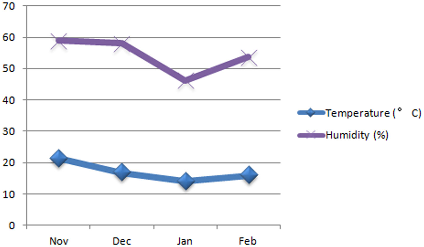
[26]	Al Shorouk City, Egypt Weather History\|Weather Underground. Available from: https://www.wunderground.com/history/monthly/eg/al-shorouk-city/HECA/date/2019-5.
[27]	Minolta K (1989) Chlorophyll meter SPAD-502 instruction manual. Available from: https://www.konicaminolta.com/instruments/download/catalog/color/pdf/spad502plus_catalog_eng.pdf.
[28]	Liu X, Huang B (2000) Heat stress injury in relation to membrane lipid peroxidation in creeping bentgrass. Crop Sci 40: 503-510. doi: 10.2135/cropsci2000.402503x
[29]	Goudarzi M, Pakniyat H (2008) Evaluation of wheat cultivars under salinity stress based on some agronomic and physiological traits. J Agri Soc Sci 4: 4.
[30]	Steel RG (1997) Pinciples and procedures of statistics a biometrical approach.
[31]	Falconer DS (1989) Introduction to quantitative genetics 3rd ed.. Harlow Longman Sci Tech .
[32]	Nadarajan N (2005) Quantitative genetics and biometrical techniques in plant breeding Kalyani Publishers.
[33]	Allard RW (1999) Principles of plant breeding John Wiley & Sons.
[34]	JOHNSON H (1955) Estimates of genetic and environmental variability in soybeans. Agron J 47: 314-318. doi: 10.2134/agronj1955.00021962004700070009x
[35]	Miles AG (1992) Biological Nitrogen Fixation Springer Science & Business Media.
[36]	Anzai Y, Kim H, Park JY, et al. (2000) Phylogenetic affiliation of the pseudomonads based on 16S rRNA sequence. Int J Syst Evol Microbiol 50: 1563-1589. doi: 10.1099/00207713-50-4-1563
[37]	Solanki MK, Wang Z, Wang FY, et al. (2017) Intercropping in sugarcane cultivation influenced the soil properties and enhanced the diversity of vital diazotrophic bacteria. Sugar Tech 19: 136-147. doi: 10.1007/s12355-016-0445-y
[38]	Santi C, Bogusz D, Franche C (2013) Biological nitrogen fixation in non-legume plants. Ann Bot 111: 743-767. doi: 10.1093/aob/mct048
[39]	Carvalho TLG, Ballesteros HGF, Thiebaut F, et al. (2016) Nice to meet you: genetic, epigenetic and metabolic controls of plant perception of beneficial associative and endophytic diazotrophic bacteria in non-leguminous plants. Plant Mol Biol 90: 561-574. doi: 10.1007/s11103-016-0435-1
[40]	Cassán F, Vanderleyden J, Spaepen S (2014) Physiological and agronomical aspects of phytohormone production by model plant-growth-promoting rhizobacteria (PGPR) belonging to the genus azospirillum. J Plant Growth Regul 33: 440-459. doi: 10.1007/s00344-013-9362-4
[41]	Verma JP, Jaiswal DK, Krishna R, et al. (2018) Characterization and screening of thermophilic Bacillus strains for developing plant growth promoting consortium from hot spring of Leh and Ladakh Region of India. Front Microbiol 9: 1293. doi: 10.3389/fmicb.2018.01293
[42]	Hussain S, Khaliq A, Matloob A, et al. (2013) Germination and growth response of three wheat cultivars to NaCl salinity. Plant Soil Environ 31: 36-43.
[43]	Wang C, Knill E, Glick BR, et al. (2000) Effect of transferring 1-aminocyclopropane-1-carboxylic acid (ACC) deaminase genes into Pseudomonas fluorescens strain CHA0 and its gacA derivative CHA96 on their growth-promoting and disease-suppressive capacities. Can J Microbiol 46: 898-907. doi: 10.1139/w00-071
[44]	Glick BR, Jacobson CB, Schwarze MMK, et al. (1994) 1-Aminocyclopropane-1-carboxylic acid deaminase mutants of the plant growth promoting rhizobacterium Pseudomonas putida GR12-2 do not stimulate canola root elongation. Can J Microbiol 40: 911-915. doi: 10.1139/m94-146
[45]	Mayak S, Tirosh T, Glick BR (2004) Plant growth-promoting bacteria confer resistance in tomato plants to salt stress. Plant Physiol Biochem 42: 565-572. doi: 10.1016/j.plaphy.2004.05.009
[46]	Kaya MD, Ipek A (2003) Effects of different soil salinity levels on germination and seedling growth of safflower (Carthamus tinctorius L.). Turk J Agric For 27: 221-227.
[47]	El-Shraiy AM, Hegazi AM, Hikal MS (2016) Nodule formation, antioxidant enzymes activities and other biochemical changes in salt stressed faba bean plants treated with glycine betaine, arbuscular mycorrhiza fungi and yeast extract. Middle East J Appl Sci 6: 1076-1099.
[48]	Egamberdieva D (2009) Alleviation of salt stress by plant growth regulators and IAA producing bacteria in wheat. Acta Physiol Plant 31: 861-864. doi: 10.1007/s11738-009-0297-0
[49]	Tiwari S, Singh P, Tiwari R, et al. (2011) Salt-tolerant rhizobacteria-mediated induced tolerance in wheat (Triticum aestivum) and chemical diversity in rhizosphere enhance plant growth. Biol Fertil Soils 47: 907. doi: 10.1007/s00374-011-0598-5
[50]	Ansari FA, Ahmad I (2018) Plant growth promoting attributes and alleviation of salinity stress to wheat by biofilm forming Brevibacterium sp. FAB3 isolated from rhizospheric soil. Saudi J Biol Sci .
[51]	Gange AC, Gadhave KR (2018) Plant growth-promoting rhizobacteria promote plant size inequality. Sci Rep 8: 13828. doi: 10.1038/s41598-018-32111-z
[52]	Glick BR, Penrose DM, Li J (1998) A model for the lowering of plant ethylene concentrations by plant growth-promoting bacteria. J Theor Biol 190: 63-68. doi: 10.1006/jtbi.1997.0532
[53]	Saravanakumar D, Samiyappan R (2007) ACC deaminase from Pseudomonas fluorescens mediated saline resistance in groundnut (Arachis hypogea) plants. J Appl Microbiol 102: 1283-1292. doi: 10.1111/j.1365-2672.2006.03179.x
[54]	Etesami H, Beattie GA (2018) Mining halophytes for plant growth-promoting halotolerant bacteria to enhance the salinity tolerance of non-halophytic crops. Front Microbiol 9: 148. doi: 10.3389/fmicb.2018.00148
[55]	Pushpavalli R, Quealy J, Colmer TD, et al. (2016) Salt stress delayed flowering and reduced reproductive success of chickpea (Cicer arietinum L.), a response associated with Na+ accumulation in leaves. J Agron Crop Sci 202: 125-138. doi: 10.1111/jac.12128
[56]	Pirasteh-Anosheh H, Ranjbar G, Pakniyat H, et al. (2015) Physiological mechanisms of salt stress tolerance in plants. Plant-Environment Interaction John Wiley & Sons, Ltd, 141-160. doi: 10.1002/9781119081005.ch8
[57]	El-Hendawy SE, Hu Y, Schmidhalter U (2007) Assessing the suitability of various physiological traits to screen wheat genotypes for salt tolerance. J Integr Plant Biol 49: 1352-1360. doi: 10.1111/j.1744-7909.2007.00533.x
[58]	KHAN MA (2009) Role of proline, K/Na ratio and chlorophyll content in salt tolerance of wheat (Triticum aestivum L.). Pak J Bot 41: 633-638.
[59]	Arkus KAJ, Cahoon EB, Jez JM (2005) Mechanistic analysis of wheat chlorophyllase. Arch Biochem Biophys 438: 146-155. doi: 10.1016/j.abb.2005.04.019
[60]	Mishra S, Tyagi A, Singh IV, et al. (2006) Changes in lipid profile during growth and senescence of Catharanthus roseus leaf. Braz J Plant Physiol 18: 447-454. doi: 10.1590/S1677-04202006000400002
[61]	Kaur P, Kaur J, Kaur S, et al. (2014) Salinity induced physiological and biochemical changes in chickpea (Cicer arietinum L.) genotypes. J Appl Nat Sci 6: 578-588. doi: 10.31018/jans.v6i2.500
[62]	Mahlooji M, Seyed Sharifi R, Razmjoo J, et al. (2018) Effect of salt stress on photosynthesis and physiological parameters of three contrasting barley genotypes. Photosynthetica 56: 549-556. doi: 10.1007/s11099-017-0699-y
[63]	Harinasut P, Poonsopa D, Roengmongkol K, et al. (2003) Salinity effects on antioxidant enzymes in mulberry cultivar. Sci Asia 29: 109-113. doi: 10.2306/scienceasia1513-1874.2003.29.109
[64]	Katsuhara M, Otsuka T, Ezaki B (2005) Salt stress-induced lipid peroxidation is reduced by glutathione S-transferase, but this reduction of lipid peroxides is not enough for a recovery of root growth in Arabidopsis. Plant Sci 2: 369-373. doi: 10.1016/j.plantsci.2005.03.030
[65]	Aghaleh M, Niknam V (2009) Effect of salinity on some physiological and biochemical parameters in explants of two cultivars of soybean (Glyicine max L.). J Phytol 1: 86-94.
[66]	Sreenivasulu N, Ramanjulu S, Ramachandra-Kini K, et al. (1999) Total peroxidase activity and peroxidase isoforms as modified by salt stress in two cultivars of fox-tail millet with differential salt tolerance. Plant Sci 141: 1-9. doi: 10.1016/S0168-9452(98)00204-0
[67]	Nazar R, Iqbal N, Syeed S, et al. (2011) Salicylic acid alleviates decreases in photosynthesis under salt stress by enhancing nitrogen and sulfur assimilation and antioxidant metabolism differentially in two mungbean cultivars. J Plant Physiol 168: 807-815. doi: 10.1016/j.jplph.2010.11.001
[68]	Weisany W, Sohrabi Y, Heidari G, et al. (2012) Changes in antioxidant enzymes activity and plant performance by salinity stress and zinc application in soybean (Glycine max L.). Plant Omics J 5: 60-67.
[69]	Zhang JL, Aziz M, Qiao Y, et al. (2014) Soil microbe Bacillus subtilis (GB03) induces biomass accumulation and salt tolerance with lower sodium accumulation in wheat. Crop Pasture Sci 65: 423-427. doi: 10.1071/CP13456
[70]	Fellahi Z, Hannachi A, Guendouz A, et al. (2013) Genetic variability, heritability and association studies in bread wheat (Triticum aestivum L.) genotypes. Electron J Plant Breed 4: 1161-1166.

Reader Comments

Your name:*

Email:*
© 2020 the Author(s), licensee AIMS Press. This is an open access article distributed under the terms of the Creative Commons Attribution License (http://creativecommons.org/licenses/by/4.0)