Staphylococcus aureus is one of the leading agents of nosocomial and community-acquired infections. In this study, we explored the genomic characterization of eight methicillin-resistant clinical isolates of S. aureus from Dhaka, Bangladesh. Notably, all strains were resistant to penicillin, cephalosporins, and monobactams, with partial susceptibility to meropenem and complete susceptibility to amikacin, vancomycin, and tigecycline antibiotics. The strains were found to have an average genome size of 2.73 Mbp and an average of 32.64% GC content. Multi-locus sequence typing analysis characterized the most predominant sequence type as ST361, which belongs to the clonal complex CC361. All isolates harbored the mecA gene, often linked to SCCmec_type IV variants. Multidrug resistance was attributed to efflux pumps NorA, NorC, SdrM, and LmrS alongside genes encoding beta-lactamase BlaZ and factors like ErmC and MepA. Additionally, virulence factors including adsA, sdrC, cap8D, harA, esaA, essC, isdB, geh, and lip were commonly identified. Furthermore, genes associated with heme uptake and clumping were present, highlighting their roles in S. aureus colonization and pathogenesis. Nine secondary metabolite biosynthetic gene clusters were found, of which six were common in all the strains. Numerous toxin-antitoxin systems were predicted, with ParE and ParB-like nuclease domains found to be the most prevalent toxin and antitoxin, respectively. Pan-genome analysis revealed 2007 core genes and 229 unique genes in the studied strains. Finally, the phylogenomic analysis showed that most Bangladeshi strains were grouped into two unique clades. This study provides a genomic and comparative insight into the multidrug resistance and pathogenicity of S. aureus strains, which will play a crucial role in the future antibiotic stewardship of Bangladesh.
Citation: Afia Anjum, Jarin Tabassum, Sohidul Islam, A. K. M. Imrul Hassan, Ishrat Jabeen, Sabbir R. Shuvo. Deciphering the genomic character of the multidrug-resistant Staphylococcus aureus from Dhaka, Bangladesh[J]. AIMS Microbiology, 2024, 10(4): 833-858. doi: 10.3934/microbiol.2024036
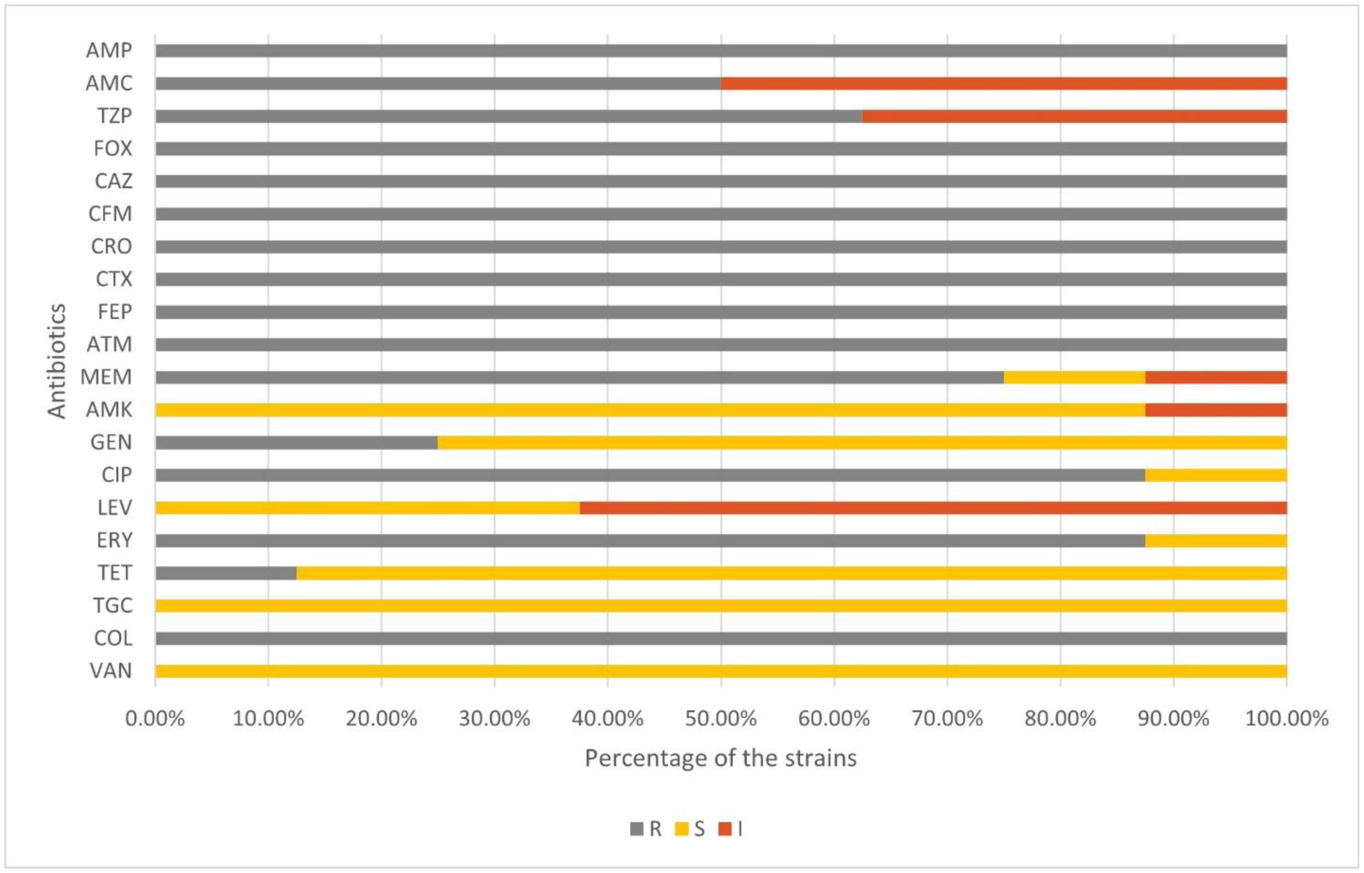
Staphylococcus aureus is one of the leading agents of nosocomial and community-acquired infections. In this study, we explored the genomic characterization of eight methicillin-resistant clinical isolates of S. aureus from Dhaka, Bangladesh. Notably, all strains were resistant to penicillin, cephalosporins, and monobactams, with partial susceptibility to meropenem and complete susceptibility to amikacin, vancomycin, and tigecycline antibiotics. The strains were found to have an average genome size of 2.73 Mbp and an average of 32.64% GC content. Multi-locus sequence typing analysis characterized the most predominant sequence type as ST361, which belongs to the clonal complex CC361. All isolates harbored the mecA gene, often linked to SCCmec_type IV variants. Multidrug resistance was attributed to efflux pumps NorA, NorC, SdrM, and LmrS alongside genes encoding beta-lactamase BlaZ and factors like ErmC and MepA. Additionally, virulence factors including adsA, sdrC, cap8D, harA, esaA, essC, isdB, geh, and lip were commonly identified. Furthermore, genes associated with heme uptake and clumping were present, highlighting their roles in S. aureus colonization and pathogenesis. Nine secondary metabolite biosynthetic gene clusters were found, of which six were common in all the strains. Numerous toxin-antitoxin systems were predicted, with ParE and ParB-like nuclease domains found to be the most prevalent toxin and antitoxin, respectively. Pan-genome analysis revealed 2007 core genes and 229 unique genes in the studied strains. Finally, the phylogenomic analysis showed that most Bangladeshi strains were grouped into two unique clades. This study provides a genomic and comparative insight into the multidrug resistance and pathogenicity of S. aureus strains, which will play a crucial role in the future antibiotic stewardship of Bangladesh.

| [1] |
Tong SYC, Davis JS, Eichenberger E, et al. (2015) Staphylococcus aureus infections: Epidemiology, pathophysiology, clinical manifestations, and management. Clin Microbiol Rev 28: 603-661. https://doi.org/10.1128/CMR.00134-14 
|
| [2] |
Self WH, Wunderink RG, Williams DJ, et al. (2016) Staphylococcus aureus community-acquired pneumonia: prevalence, clinical characteristics, and outcomes. Clin Infect Dis 63: 300-309. https://doi.org/10.1093/CID/CIW300
|
| [3] |
Grapsa J, Blauth C, Chandrashekhar YS, et al. (2022) Staphylococcus aureus infective endocarditis: jacc patient pathways. JACC Case Reports 4: 1-12. https://doi.org/10.1016/J.JACCAS.2021.10.002
|
| [4] |
Kwiecinski JM, Horswill AR (2020) Staphylococcus aureus bloodstream infections: pathogenesis and regulatory mechanisms. Curr Opin Microbiol 53: 51-60. https://doi.org/10.1016/J.MIB.2020.02.005
|
| [5] |
Malachowa N, Deleo FR (2010) Mobile genetic elements of Staphylococcus aureus. Cell Mol Life Sci 67: 3057-3071. https://doi.org/10.1007/s00018-010-0389-4
|
| [6] | Islam T, Kubra K, Hassan Chowdhury MM (2018) Prevalence of methicillin-resistant Staphylococcus aureus in Hospitals in Chittagong, Bangladesh: A threat of nosocomial infection. J Microsc Ultrastruct 6: 188-191. https://doi.org/10.4103/JMAU.JMAU_33_18 |
| [7] |
Kayili E, Sanlibaba P (2020) Prevalence, characterization and antibiotic resistance of Staphylococcus aureus isolated from traditional cheeses in Turkey. Int J Food Prop 23: 1441-1451. https://doi.org/10.1080/10942912.2020.1814323
|
| [8] |
Loomba P, Taneja J, Mishra B (2010) Methicillin and vancomycin resistant S. aureus in hospitalized patients. J Glob Infect Dis 2: 275-283. https://doi.org/10.4103/0974-777x.68535
|
| [9] |
Kali A (2015) Antibiotics and bioactive natural products in treatment of methicillin resistant Staphylococcus aureus: a brief review. Pharmacogn Rev 9: 29-34. https://doi.org/10.4103/0973-7847.156329
|
| [10] | Abdallah EM, Mohamed Abdallah E (2016) Medicinal plants as an alternative drug against methicillin resistant Staphylococcus aureus. Int J Microbiol Allied Sci 3: 35-42. |
| [11] |
Zhang K, McClure JA, Elsayed S, et al. (2009) Novel staphylococcal cassette chromosome mec type, tentatively designated type VIII, harboring class A mec and type 4 ccr gene complexes in a Canadian epidemic strain of methicillin-resistant Staphylococcus aureus. Antimicrob Agents Chemother 53: 531-540. https://doi.org/10.1128/AAC.01118-08
|
| [12] |
Foster TJ (2017) Antibiotic resistance in Staphylococcus aureus. Current status and future prospects. FEMS Microbiol Rev 41: 430-449. https://doi.org/10.1093/FEMSRE/FUX007
|
| [13] |
Hou Z, Liu L, Wei J, et al. (2023) Progress in the prevalence, classification and drug resistance mechanisms of methicillin-resistant Staphylococcus aureus. Infect Drug Resist 16: 3271-3292. https://doi.org/10.2147/IDR.S412308
|
| [14] | Geoghegan JA, Foster TJ (2017) Cell wall-anchored surface proteins of Staphylococcus aureus: Many proteins, multiple functions. Current Topics in Microbiology and Immunology . Springer Verlag 95-120. https://doi.org/10.1007/82_2015_5002 |
| [15] |
Foster TJ, Geoghegan JA, Ganesh VK, et al. (2014) Adhesion, invasion and evasion: The many functions of the surface proteins of Staphylococcus aureus. Nat Rev Microbiol 12: 49-62. https://doi.org/10.1038/nrmicro3161
|
| [16] | Tam K, Torres VJ (2019) Staphylococcus aureus secreted toxins and extracellular enzymes. Microbiol Spectr 7. https://doi.org/10.1128/microbiolspec.gpp3-0039-2018 |
| [17] | Yusuf MA, Islam S, Shamsuzzaman A, et al. (2013) Burden of infection caused by methicillin-resistant Staphylococcus aureus in Bangladesh: a systematic review. Glob Adv Res J Microbiol 2: 213-223. |
| [18] |
Nickerson EK, West TE, Day NP, et al. (2009) Staphylococcus aureus disease and drug resistance in resource-limited countries in south and east Asia. Lancet Infect Dis 9: 130-135. https://doi.org/10.1016/S1473-3099(09)70022-2
|
| [19] |
Chongtrakool P, Ito T, Ma XX, et al. (2006) Staphylococcal cassette chromosome mec (SCCmec) typing of methicillin-resistant Staphylococcus aureus strains isolated in 11 Asian countries: A proposal for a new nomenclature for SCCmec elements. Antimicrob Agents Chemother 50: 1001-1012. https://doi.org/10.1128/AAC.50.3.1001-1012.2006
|
| [20] |
Hussain K, Rahman M, Nazir KHMNH, et al. (2016) Methicillin pesistant Staphylococcus aureus (MRSA) in Patients of Community Based Medical College Hospital, Mymensingh, Bangladesh. Am J Biomed Life Sci 4: 26-29. https://doi.org/10.11648/j.ajbls.20160403.11
|
| [21] | Roy S, Barman TK, Hossain MA, et al. (2017) Molecular-characterization of methicillin-resistance Staphylococcus aureus (MRSA) from different Tertiary Care Hospitals in Bangladesh. Mymensingh Med J 26: 37-44. |
| [22] |
Rahman MM, Amin KB, Rahman SMM, et al. (2018) Investigation of methicillin-resistant Staphylococcus aureus among clinical isolates from humans and animals by culture methods and multiplex PCR. BMC Vet Res 14: 300. https://doi.org/10.1186/s12917-018-1611-0
|
| [23] |
Jorgensen JH, Turnidge JD (2015) Susceptibility test methods: dilution and disk diffusion methods. Manual of Clinical Microbiology . John Wiley & Sons, Ltd 1253-1273. https://doi.org/10.1128/9781555817381.ch71
|
| [24] | CLSIM100-performance standards for antimicrobial susceptibility testing, clinical and laboratory standards institute (2022). |
| [25] |
Magiorakos AP, Srinivasan A, Carey RB, et al. (2012) Multidrug-resistant, extensively drug-resistant and pandrug-resistant bacteria: An international expert proposal for interim standard definitions for acquired resistance. Clin Microbiol Infect 18: 268-281. https://doi.org/10.1111/j.1469-0691.2011.03570.x
|
| [26] |
Stepanović S, Vuković D, Dakić I, et al. (2000) A modified microtiter-plate test for quantification of staphylococcal biofilm formation. J Microbiol Methods 40: 175-179. https://doi.org/10.1016/S0167-7012(00)00122-6
|
| [27] |
Wick RR, Judd LM, Gorrie CL, et al. (2017) Unicycler: Resolving bacterial genome assemblies from short and long sequencing reads. PLoS Comput Biol 13: e1005595. https://doi.org/10.1371/journal.pcbi.1005595
|
| [28] |
Li H, Handsaker B, Wysoker A, et al. (2009) The sequence alignment/map format and SAMtools. Bioinformatics 25: 2078-2079. https://doi.org/10.1093/BIOINFORMATICS/BTP352
|
| [29] |
Gurevich A, Saveliev V, Vyahhi N, et al. (2013) QUAST: Quality assessment tool for genome assemblies. Bioinformatics 29: 1072-1075. https://doi.org/10.1093/bioinformatics/btt086
|
| [30] |
Brettin T, Davis JJ, Disz T, et al. (2015) RASTtk: A modular and extensible implementation of the RAST algorithm for building custom annotation pipelines and annotating batches of genomes. Sci Rep 5: 8365. https://doi.org/10.1038/srep08365
|
| [31] |
Olson RD, Assaf R, Brettin T, et al. (2023) Introducing the bacterial and viral bioinformatics resource center (BV-BRC): a resource combining PATRIC, IRD and ViPR. Nucleic Acids Res 51: D678-D689. https://doi.org/10.1093/NAR/GKAC1003
|
| [32] |
Wattam AR, Davis JJ, Assaf R, et al. (2017) Improvements to PATRIC, the all-bacterial bioinformatics database and analysis resource center. Nucleic Acids Res 45: D535-D542. https://doi.org/10.1093/nar/gkw1017
|
| [33] |
Grant JR, Enns E, Marinier E, et al. (2023) Proksee: In-depth characterization and visualization of bacterial genomes. Nucleic Acids Res 51: W484-W492. https://doi.org/10.1093/nar/gkad326
|
| [34] |
Alcock BP, Huynh W, Chalil R, et al. (2023) CARD 2023: expanded curation, support for machine learning, and resistome prediction at the Comprehensive Antibiotic Resistance Database. Nucleic Acids Res 51: D690-D699. https://doi.org/10.1093/NAR/GKAC920
|
| [35] |
Ito T, Hiramatsu K, Oliveira DC, et al. (2009) Classification of staphylococcal cassette chromosome mec (SCCmec): Guidelines for reporting novel SCCmec elements. Antimicrob Agents Chemother 53: 4961-4967. https://doi.org/10.1128/AAC.00579-09
|
| [36] |
Kondo Y, Ito T, Ma XX, et al. (2007) Combination of multiplex PCRs for staphylococcal cassette chromosome mec type assignment: Rapid identification system for mec, ccr, and major differences in junkyard regions. Antimicrob Agents Chemother 51: 264-274. https://doi.org/10.1128/AAC.00165-06
|
| [37] |
Camacho C, Coulouris G, Avagyan V, et al. (2009) BLAST+: Architecture and applications. BMC Bioinformatics 10: 421. https://doi.org/10.1186/1471-2105-10-421
|
| [38] |
Larsen MV, Cosentino S, Rasmussen S, et al. (2012) Multilocus sequence typing of total-genome-sequenced bacteria. J Clin Microbiol 50: 1355-1361. https://doi.org/10.1128/JCM.06094-11
|
| [39] |
Griffiths D, Fawley W, Kachrimanidou M, et al. (2010) Multilocus sequence typing of Clostridium difficile. J Clin Microbiol 48: 770-778. https://doi.org/10.1128/JCM.01796-09
|
| [40] |
Jolley KA, Bray JE, Maiden MCJ (2018) Open-access bacterial population genomics: BIGSdb software, the PubMLST.org website and their applications. Wellcome Open Res 3: 124. https://doi.org/10.12688/wellcomeopenres.14826.1
|
| [41] |
Bartels MD, Petersen A, Worning P, et al. (2014) Comparing whole-genome sequencing with sanger sequencing for spa typing of methicillin-resistant Staphylococcus aureus. J Clin Microbiol 52: 4305-4308. https://doi.org/10.1128/JCM.01979-14
|
| [42] |
Cosentino S, Voldby Larsen M, Møller Aarestrup F, et al. (2013) PathogenFinder-distinguishing friend from foe using bacterial whole genome sequence data. PLoS One 8: e77302. https://doi.org/10.1371/journal.pone.0077302
|
| [43] |
Carattoli A, Zankari E, Garciá-Fernández A, et al. (2014) In Silico detection and typing of plasmids using plasmidfinder and plasmid multilocus sequence typing. Antimicrob Agents Chemother 58: 3895-3903. https://doi.org/10.1128/AAC.02412-14
|
| [44] |
Arndt D, Grant JR, Marcu A, et al. (2016) PHASTER: a better, faster version of the PHAST phage search tool. Nucleic Acids Res 44: W16-W21. https://doi.org/10.1093/nar/gkw387
|
| [45] |
Zhou Y, Liang Y, Lynch KH, et al. (2011) PHAST: A fast phage search tool. Nucleic Acids Res 39: W347-W352. https://doi.org/10.1093/nar/gkr485
|
| [46] |
Liu M, Li X, Xie Y, et al. (2019) ICEberg 2.0: An updated database of bacterial integrative and conjugative elements. Nucleic Acids Res 47: D660-D665. https://doi.org/10.1093/nar/gky1123
|
| [47] |
Chen L, Yang J, Yu J, et al. (2005) VFDB: a reference database for bacterial virulence factors. Nucleic Acids Res 33: D325-D328. https://doi.org/10.1093/NAR/GKI008
|
| [48] |
Blin K, Shaw S, Augustijn HE, et al. (2023) antiSMASH 7.0: new and improved predictions for detection, regulation, chemical structures and visualisation. Nucleic Acids Res 51: W46-W50. https://doi.org/10.1093/NAR/GKAD344
|
| [49] |
Akarsu H, Bordes P, Mansour M, et al. (2019) TASmania: A bacterial Toxin-Antitoxin Systems database. PLOS Comput Biol 15: e1006946. https://doi.org/10.1371/JOURNAL.PCBI.1006946
|
| [50] |
Chaudhari NM, Gupta VK, Dutta C (2016) BPGA-an ultra-fast pan-genome analysis pipeline. Sci Rep 6: 24373. https://doi.org/10.1038/srep24373
|
| [51] | Rodriguez-R LM, Konstantinidis KT (2016) The enveomics collection: a toolbox for specialized analyses of microbial genomes and metagenomes. PeerJ Prepr 4: e1900v1. https://doi.org/10.7287/PEERJ.PREPRINTS.1900V1 |
| [52] |
Meier-Kolthoff JP, Göker M (2019) TYGS is an automated high-throughput platform for state-of-the-art genome-based taxonomy. Nat Commun 10: 2182. https://doi.org/10.1038/s41467-019-10210-3
|
| [53] |
Kaas RS, Leekitcharoenphon P, Aarestrup FM, et al. (2014) Solving the problem of comparing whole bacterial genomes across different sequencing platforms. PLoS One 9: e104984. https://doi.org/10.1371/JOURNAL.PONE.0104984
|
| [54] |
Letunic I, Bork P (2021) Interactive Tree Of Life (iTOL) v5: an online tool for phylogenetic tree display and annotation. Nucleic Acids Res 49: W293-W296. https://doi.org/10.1093/NAR/GKAB301
|
| [55] |
Alam FM, Tasnim T, Afroz S, et al. (2023) Epidemiology and antibiogram of clinical Staphylococcus aureus isolates from Tertiary Care Hospitals in Dhaka, Bangladesh. Avicenna J Clin Microbiol Infect 9: 137-147. https://doi.org/10.34172/AJCMI.2022.3391
|
| [56] |
Haque N, Aung MS, Paul SK, et al. (2019) Molecular epidemiological characterization of methicillin-susceptible and -resistant Staphylococcus aureus isolated from skin and soft tissue infections in Bangladesh. Microb Drug Resist 25: 241-250. https://doi.org/10.1089/mdr.2018.0123
|
| [57] |
Mairi A, Touati A, Lavigne JP (2020) Methicillin-resistant Staphylococcus aureus ST80 Clone: A systematic review. Toxins 12: 119. https://doi.org/10.3390/toxins12020119
|
| [58] |
Sarkhoo E, Udo EE, Boswihi SS, et al. (2021) The dissemination and molecular characterization of clonal complex 361 (CC361) methicillin-resistant Staphylococcus aureus (MRSA) in Kuwait Hospitals. Front Microbiol 12: 658772. https://doi.org/10.3389/fmicb.2021.658772
|
| [59] |
Islam MA, Parveen S, Rahman M, et al. (2019) Occurrence and characterization of methicillin resistant Staphylococcus aureus in processed raw foods and ready-to-eat foods in an urban setting of a developing country. Front Microbiol 10: 503. https://doi.org/10.3389/FMICB.2019.00503
|
| [60] |
Kinnevey PM, Shore AC, Brennan GI, et al. (2014) Extensive genetic diversity identified among sporadic methicillin-resistant Staphylococcus aureus isolates recovered in Irish hospitals between 2000 and 2012. Antimicrob Agents Chemother 58: 1907-1917. https://doi.org/10.1128/AAC.02653-13
|
| [61] |
Boswihi SS, Udo EE, Al-Sweih N (2016) Shifts in the clonal distribution of methicillin-resistant Staphylococcus aureus in Kuwait Hospitals: 1992-2010. PLoS One 11: e0162744. https://doi.org/10.1371/journal.pone.0162744
|
| [62] |
Afroz S, Kobayashi N, Nagashima S, et al. (2008) Genetic characterization of Staphylococcus aureus isolates carrying Panton-Valentine leukocidin genes in Bangladesh. Jpn J Infect Dis 61: 393-396. https://doi.org/10.7883/yoken.jjid.2008.393
|
| [63] | Weber S, Ehricht R, Slickers P (2010) Genetic fingerprinting of MRSA from Abu Dhabi. ECCMID . |
| [64] | Martínez-Meléndez A, Morfín-Otero R, Villarreal-Treviño L, et al. (2015) Staphylococcal Cassette Chromosome mec (SCCmec) in coagulase negative staphylococci. Med Univ 17: 229-233. https://doi.org/10.1016/J.RMU.2015.10.003 |
| [65] |
Liakopoulos A, Foka A, Vourli S, et al. (2011) Aminoglycoside-resistant staphylococci in Greece: Prevalence and resistance mechanisms. Eur J Clin Microbiol Infect Dis 30: 701-705. https://doi.org/10.1007/s10096-010-1132-7
|
| [66] | Khoramrooz SS, Alipoor Dolatabad S, Mostafapour Dolatabad F, et al. (2017) Detection of tetracycline resistance genes, aminoglycoside modifying enzymes, and coagulase gene typing of clinical isolates of Staphylococcus aureus in the Southwest of Iran. Iran J Basic Med Sci 20: 912-919. https://doi.org/10.22038/IJBMS.2017.9114 |
| [67] |
Becker B, Cooper MA (2013) Aminoglycoside antibiotics in the 21st century. ACS Chem Biol 8: 105-115. https://doi.org/10.1021/CB3005116
|
| [68] |
Floyd JL, Smith KP, Kumar SH, et al. (2010) LmrS is a multidrug efflux pump of the major facilitator superfamily from Staphylococcus aureus. Antimicrob Agents Chemother 54: 5406-5412. https://doi.org/10.1128/AAC.00580-10
|
| [69] |
Costa SS, Sobkowiak B, Parreira R, et al. (2019) Genetic diversity of norA, coding for a main efflux pump of Staphylococcus aureus. Front Genet 9: 710. https://doi.org/10.3389/fgene.2018.00710
|
| [70] |
Silva KPT, Sundar G, Khare A (2023) Efflux pump gene amplifications bypass necessity of multiple target mutations for resistance against dual-targeting antibiotic. Nat Commun 14: 3402. https://doi.org/10.1038/s41467-023-38507-4
|
| [71] |
Sandvik EL, Fazen CH, Henry TC, et al. (2015) Non-monotonic survival of Staphylococcus aureus with respect to ciprofloxacin concentration arises from prophage-dependent killing of persisters. Pharmaceuticals 8: 778-792. https://doi.org/10.3390/ph8040778
|
| [72] |
Lai CC, Chen CC, Lu YC, et al. (2018) The clinical significance of silent mutations with respect to ciprofloxacin resistance in MRSA. Infect Drug Resist 11: 681-687. https://doi.org/10.2147/IDR.S159455
|
| [73] |
Hyun JC, Kavvas ES, Monk JM, et al. (2020) Machine learning with random subspace ensembles identifies antimicrobial resistance determinants from pan-genomes of three pathogens. PLOS Comput Biol 16: e1007608. https://doi.org/10.1371/JOURNAL.PCBI.1007608
|
| [74] |
Huang H, Wan P, Luo X, et al. (2023) Tigecycline resistance-associated mutations in the mepa efflux pump in Staphylococcus aureus. Microbiol Spectr 11: e0063423. https://doi.org/10.1128/spectrum.00634-23
|
| [75] |
Zeng W, Zhang X, Liu Y, et al. (2022) In vitro antimicrobial activity and resistance mechanisms of the new generation tetracycline agents, eravacycline, omadacycline, and tigecycline against clinical Staphylococcus aureus isolates. Front Microbiol 13: 1043736. https://doi.org/10.3389/fmicb.2022.1043736
|
| [76] |
Dashtbani-Roozbehani A, Brown MH (2021) Efflux pump mediated antimicrobial resistance by staphylococci in health-related environments: Challenges and the quest for inhibition. Antibiotics 10: 1502. https://doi.org/10.3390/antibiotics10121502
|
| [77] |
Miklasińska-Majdanik M (2021) Mechanisms of resistance to macrolide antibiotics among Staphylococcus aureus. Antibiotics 10: 1406. https://doi.org/10.3390/antibiotics10111406
|
| [78] |
Rowe SJ, Mecaskey RJ, Nasef M, et al. (2020) Shared requirements for key residues in the antibiotic resistance enzymes ErmC and ErmE suggest a common mode of RNA recognition. J Biol Chem 295: 17476-17485. https://doi.org/10.1074/jbc.RA120.014280
|
| [79] | Duran N, Ozer B, Duran GG, et al. (2012) Antibiotic resistance genes & susceptibility patterns in staphylococci. Indian J Med Res 135: 389-396. |
| [80] |
Aziz KE, Abdulrahman ZFA (2021) Detection of tetracycline tet(k) gene in clinical Staphylococcus aureus isolates. IOP Conf Ser Earth Environ Sci 761: 012128. https://doi.org/10.1088/1755-1315/761/1/012128
|
| [81] |
You Y, Hilpert M, Ward MJ (2013) Identification of Tet45, a tetracycline efflux pump, from a poultry-litter-exposed soil isolate and persistence of tet(45) in the soil. J Antimicrob Chemother 68: 1962-1969. https://doi.org/10.1093/JAC/DKT127
|
| [82] |
Truong-Bolduc QC, Villet RA, Estabrooks ZA, et al. (2014) Native efflux pumps contribute resistance to antimicrobials of skin and the ability of Staphylococcus aureus to colonize skin. J Infect Dis 209: 1485-1493. https://doi.org/10.1093/infdis/jit660
|
| [83] |
Chen C, Hooper DC (2018) Effect of Staphylococcus aureus Tet38 native efflux pump on in vivo response to tetracycline in a murine subcutaneous abscess model. J Antimicrob Chemother 73: 720-723. https://doi.org/10.1093/jac/dkx432
|
| [84] |
Vestergaard M, Nøhr-Meldgaard K, Bojer MS, et al. (2017) Inhibition of the ATP synthase eliminates the intrinsic resistance of Staphylococcus aureus towards polymyxins. MBio 8: e01114-17. https://doi.org/10.1128/mBio.01114-17
|
| [85] |
Thompson MK, Keithly ME, Goodman MC, et al. (2014) Structure and function of the genomically encoded fosfomycin resistance enzyme, FosB, from Staphylococcus aureus. Biochemistry 53: 755-765. https://doi.org/10.1021/bi4015852
|
| [86] |
Chen Y, Ji S, Sun L, et al. (2022) The novel fosfomycin resistance gene fosY is present on a genomic island in CC1 methicillin-resistant Staphylococcus aureus. Emerg Microbes Infect 11: 1166-1173. https://doi.org/10.1080/22221751.2022.2058421
|
| [87] |
Nurjadi D, Schäfer J, Friedrich-Jänicke B, et al. (2015) Predominance of dfrG as determinant of trimethoprim resistance in imported Staphylococcus aureus. Clin Microbiol Infect 21: 1095.e5-1095.e9. https://doi.org/10.1016/j.cmi.2015.08.021
|
| [88] |
Pishchany G, Sheldon JR, Dickson CF, et al. (2014) IsdB-dependent hemoglobin binding is required for acquisition of heme by Staphylococcus aureus. J Infect Dis 209: 1764-1772. https://doi.org/10.1093/INFDIS/JIT817
|
| [89] |
Shambat S, Nadig S, Prabhakara S, et al. (2012) Clonal complexes and virulence factors of Staphylococcus aureus from several cities in India. BMC Microbiol 12: 64. https://doi.org/10.1186/1471-2180-12-64
|
| [90] |
Beceiro A, Tomás M, Bou G (2013) Antimicrobial resistance and virulence: A successful or deleterious association in the bacterial world?. Clin Microbiol Rev 26: 185-230. https://doi.org/10.1128/CMR.00059-12
|
| [91] |
Ruiz B, Chávez A, Forero A, et al. (2010) Production of microbial secondary metabolites: Regulation by the carbon source. Crit Rev Microbiol 36: 146-167. https://doi.org/10.3109/10408410903489576
|
| [92] | Grim KP, Radin JN, Solórzano PKP, et al. (2020) Intracellular accumulation of staphylopine can sensitize Staphylococcus aureus to host-imposed zinc starvation by chelation-independent toxicity. J Bacteriol 202: e00014-20. https://doi.org/10.1128/JB.00014-20 |
| [93] |
Chen C, Hooper DC (2019) Intracellular accumulation of Staphylopine impairs the fitness of Staphylococcus aureus cntE mutant. FEBS Lett 593: 1213-1222. https://doi.org/10.1002/1873-3468.13396
|
| [94] |
Dale SE, Doherty-Kirby A, Lajoie G, et al. (2004) Role of siderophore biosynthesis in virulence of Staphylococcus aureus: identification and characterization of genes involved in production of a siderophore. Infect Immun 72: 29-37. https://doi.org/10.1128/IAI.72.1.29-37.2004
|
| [95] |
Tripathi A, Schofield MM, Chlipala GE, et al. (2014) Baulamycins A and B, broad-spectrum antibiotics identified as inhibitors of siderophore biosynthesis in Staphylococcus aureus and Bacillus anthracis. J Am Chem Soc 136: 1579-1586. https://doi.org/10.1021/ja4115924
|
| [96] |
Grim KP, San Francisco B, Radin JN, et al. (2017) The metallophore staphylopine enables Staphylococcus aureus to compete with the host for zinc and overcome nutritional immunity. MBio 8: e01281-17. https://doi.org/10.1128/mBio.01281-17
|
| [97] |
Ghssein G, Ezzeddine Z (2022) The key element role of metallophores in the pathogenicity and virulence of Staphylococcus aureus: A review. Biology 11: 1525. https://doi.org/10.3390/biology11101525
|
| [98] |
Parvez A, Giri S, Giri GR, et al. (2018) Novel type iii polyketide synthases biosynthesize methylated polyketides in Mycobacterium marinum. Sci Rep 8: 6529. https://doi.org/10.1038/s41598-018-24980-1
|
| [99] |
Sun F, Cho H, Jeong DW, et al. (2010) Aureusimines in Staphylococcus aureus Are Not Involved in Virulence. PLoS One 5: e15703. https://doi.org/10.1371/journal.pone.0015703
|
| [100] |
Barbosa J, Caetano T, Mendo S (2015) Class I and Class II lanthipeptides produced by Bacillus spp. J Nat Prod 78: 2850-2866. https://doi.org/10.1021/np500424y
|
| [101] |
Hudson GA, Mitchell DA (2018) RiPP antibiotics: biosynthesis and engineering potential. Curr Opin Microbiol 45: 61-69. https://doi.org/10.1016/j.mib.2018.02.010
|
| [102] |
Stariha LM, McCafferty DG (2021) Discovery of the Class I antimicrobial lasso peptide arcumycin. ChemBioChem 22: 2632-2640. https://doi.org/10.1002/CBIC.202100132
|
| [103] |
Kamruzzaman M, Iredell J (2019) A ParDE-family toxin antitoxin system in major resistance plasmids of Enterobacteriaceae confers antibiotic and heat tolerance. Sci Rep 9: 9872. https://doi.org/10.1038/s41598-019-46318-1
|
| [104] |
Maisonneuve E, Shakespeare LJ, Jørgensen MG, et al. (2011) Bacterial persistence by RNA endonucleases. Proc Natl Acad Sci USA 108: 13206-13211. https://doi.org/10.1073/pnas.1100186108
|
| [105] |
Dörr T, Vulić M, Lewis K (2010) Ciprofloxacin causes persister formation by inducing the TisB toxin in Escherichia coli. PLOS Biol 8: e1000317. https://doi.org/10.1371/JOURNAL.PBIO.1000317
|
| [106] |
Schuster CF, Bertram R (2013) Toxin–antitoxin systems are ubiquitous and versatile modulators of prokaryotic cell fate. FEMS Microbiol Lett 340: 73-85. https://doi.org/10.1111/1574-6968.12074
|
| [107] |
Mruk I, Kobayashi I (2014) To be or not to be: Regulation of restriction-modification systems and other toxin-antitoxin systems. Nucleic Acids Res 42: 70-86. https://doi.org/10.1093/nar/gkt711
|
| [108] |
Schuster CF, Bertram R (2016) Toxin-antitoxin systems of Staphylococcus aureus. Toxins 8: 140. https://doi.org/10.3390/toxins8050140
|
| [109] |
Motyka-Pomagruk A, Zoledowska S, Misztak AE, et al. (2020) Comparative genomics and pangenome-oriented studies reveal high homogeneity of the agronomically relevant enterobacterial plant pathogen Dickeya solani. BMC Genomics 21: 449. https://doi.org/10.1186/s12864-020-06863-w
|
| [110] |
Sivakumar R, Pranav PS, Annamanedi M, et al. (2023) Genome sequencing and comparative genomic analysis of bovine mastitis-associated Staphylococcus aureus strains from India. BMC Genomics 24: 44. https://doi.org/10.1186/s12864-022-09090-7
|
 microbiol-10-04-036-s001.pdf microbiol-10-04-036-s001.pdf |
 |


Figures(8) / Tables(3)

Afia Anjum, Jarin Tabassum, Sohidul Islam, A. K. M. Imrul Hassan, Ishrat Jabeen, Sabbir R. Shuvo. Deciphering the genomic character of the multidrug-resistant Staphylococcus aureus from Dhaka, Bangladesh[J]. AIMS Microbiology, 2024, 10(4): 833-858. doi: 10.3934/microbiol.2024036


 DownLoad: