Loading [MathJax]/jax/output/SVG/jax.js
Case report Special Issues

Geotechnical characteristics of sensitive Leda clay at Canada test site in Gloucester, Ontario

  • In 1954, the Canadian Geotechnical Research Site No. 1 was established as a testing and experimentation site for the soft and highly sensitive Leda clays that were deposited within the now-drained Champlain Sea. The Gloucester test site has a shallow groundwater table taken as hydrostatic at 0.8 m and is underlain by a sequence of leached marine sediments that make-up the Leda clays and extend about 22 m below grade. Below that are dense glacial tills and limestone bedrock. Previous research studies at the site have included full-scale construction, monitoring, and instrumentation of shallow foundations, embankments, drilled shafts, and driven pilings. Recently, a series of in-situ tests in 2012 and 2014 included type 1 and 2 piezocone soundings, porewater dissipations, and both conventional downhole tests and continuous-interval shear wave velocity measurements have been undertaken. Selected results obtained from laboratory, in-situ testing, and geophysical tests over the past six decades are presented.

    Citation: Paul W. Mayne, Ethan Cargill, Bruce Miller. Geotechnical characteristics of sensitive Leda clay at Canada test site in Gloucester, Ontario[J]. AIMS Geosciences, 2019, 5(3): 390-411. doi: 10.3934/geosci.2019.3.390

    Related Papers:

    [1] Tongyu Wang, Yadong Chen . Event-triggered control of flexible manipulator constraint system modeled by PDE. Mathematical Biosciences and Engineering, 2023, 20(6): 10043-10062. doi: 10.3934/mbe.2023441
    [2] Yunxia Wei, Yuanfei Zhang, Bin Hang . Construction and management of smart campus: Anti-disturbance control of flexible manipulator based on PDE modeling. Mathematical Biosciences and Engineering, 2023, 20(8): 14327-14352. doi: 10.3934/mbe.2023641
    [3] Xingjia Li, Jinan Gu, Zedong Huang, Chen Ji, Shixi Tang . Hierarchical multiloop MPC scheme for robot manipulators with nonlinear disturbance observer. Mathematical Biosciences and Engineering, 2022, 19(12): 12601-12616. doi: 10.3934/mbe.2022588
    [4] Kangsen Huang, Zimin Wang . Research on robust fuzzy logic sliding mode control of Two-DOF intelligent underwater manipulators. Mathematical Biosciences and Engineering, 2023, 20(9): 16279-16303. doi: 10.3934/mbe.2023727
    [5] Yongli Yan, Fucai Liu, Teng Ren, Li Ding . Nonlinear extended state observer based control for the teleoperation of robotic systems with flexible joints. Mathematical Biosciences and Engineering, 2024, 21(1): 1203-1227. doi: 10.3934/mbe.2024051
    [6] Tianqi Yu, Lei Liu, Yan-Jun Liu . Observer-based adaptive fuzzy output feedback control for functional constraint systems with dead-zone input. Mathematical Biosciences and Engineering, 2023, 20(2): 2628-2650. doi: 10.3934/mbe.2023123
    [7] Balázs Csutak, Gábor Szederkényi . Robust control and data reconstruction for nonlinear epidemiological models using feedback linearization and state estimation. Mathematical Biosciences and Engineering, 2025, 22(1): 109-137. doi: 10.3934/mbe.2025006
    [8] Siyu Li, Shu Li, Lei Liu . Fuzzy adaptive event-triggered distributed control for a class of nonlinear multi-agent systems. Mathematical Biosciences and Engineering, 2024, 21(1): 474-493. doi: 10.3934/mbe.2024021
    [9] Xinyu Shao, Zhen Liu, Baoping Jiang . Sliding-mode controller synthesis of robotic manipulator based on a new modified reaching law. Mathematical Biosciences and Engineering, 2022, 19(6): 6362-6378. doi: 10.3934/mbe.2022298
    [10] Xingjia Li, Jinan Gu, Zedong Huang, Wenbo Wang, Jing Li . Optimal design of model predictive controller based on transient search optimization applied to robotic manipulators. Mathematical Biosciences and Engineering, 2022, 19(9): 9371-9387. doi: 10.3934/mbe.2022436
  • In 1954, the Canadian Geotechnical Research Site No. 1 was established as a testing and experimentation site for the soft and highly sensitive Leda clays that were deposited within the now-drained Champlain Sea. The Gloucester test site has a shallow groundwater table taken as hydrostatic at 0.8 m and is underlain by a sequence of leached marine sediments that make-up the Leda clays and extend about 22 m below grade. Below that are dense glacial tills and limestone bedrock. Previous research studies at the site have included full-scale construction, monitoring, and instrumentation of shallow foundations, embankments, drilled shafts, and driven pilings. Recently, a series of in-situ tests in 2012 and 2014 included type 1 and 2 piezocone soundings, porewater dissipations, and both conventional downhole tests and continuous-interval shear wave velocity measurements have been undertaken. Selected results obtained from laboratory, in-situ testing, and geophysical tests over the past six decades are presented.


    Flexible manipulators, as autonomous robots, possess the capability to move and execute tasks independently without direct human intervention, as highlighted in references such as [1,2,3]. These robots are typically equipped with a range of functionalities, including autonomous navigation, environmental sensing, decision-making and execution capabilities. These features enable them to operate autonomously, navigate diverse environments, interact with their surroundings and accomplish predefined tasks. The applications of flexible manipulators are extensive, spanning various domains such as industrial automation, smart homes, agriculture, field management, exploration and search and rescue operations. They contribute to increased work efficiency, reduced labor requirements, and the ability to handle hazardous and challenging tasks effectively.

    Attitude tracking control of flexible manipulators or nonlinear systems has always been a hot research topic [4,5,6]. To address these issues, researchers have proposed various methods in the control of flexible manipulators. In [7], a disturbance observer is designed to estimate the presence of external disturbances in a flexible manipulator. Additionally, they utilize H control based on specified performance and iterative learning control techniques to address both the vibration and inertia uncertainties of the flexible manipulator while achieving good tracking performance. In [8], the study addressed the vibration suppression and angle tracking issues of a flexible unmanned aerospace system with input nonlinearity, asymmetric output constraints and uncertain system parameters. Utilizing inversion techniques, a boundary control scheme was developed to mitigate vibrations and adjust the spacecraft's angle. Simulations also demonstrated the strong robustness of this approach. In [9], researchers address the challenge of tracking desired motion trajectories within an underwater robot-manipulator system, particularly when direct velocity feedback is unavailable. To tackle this issue, a comprehensive controller-observer scheme is developed, leveraging an observer to estimate the system's velocity. This innovative approach not only achieves exponential convergence in motion tracking but also ensures a simultaneous convergence in estimation errors. Different from the References [7] and [9], Reference [10] proposes a finite-time trajectory tracking controller for space manipulators. In this context, a radial basis function neural network is utilized to both estimate and compensate for the uncertain model of the space manipulator, especially when dealing with the capture of unknown loads. An auxiliary system is designed to mitigate actuator saturation. In [11], a new adaptive control law is proposed to solve the terminal tracking problem of underwater robot-manipulator systems. In addition, using the unit quaternion to represent attitude overcomes the problem of kinematic singularity. The primary objective of this controller is to guarantee the convergence of tracking errors to zero, even in the presence of uncertainties. Furthermore, it is designed to maintain system stability and achieve satisfactory tracking performance, even when operating under underactuated conditions [12]. In essence, the proposed control strategy provides a robust and effective means to ensure precise tracking performance for the aerial manipulator system, even when facing uncertainties and underactuation challenges.

    In practical control systems, one of the most common nonlinear challenges arises from the physical characteristics of actuators, specifically, their limited output amplitude. This issue is known as the input saturation problem [13,14,15,16,17]. Furthermore, limitations in actuator control inputs refer to the existence of input restrictions in the control system of the flexible manipulator system [18,19]. This means that the actuators of the flexible manipulator, such as motors or hydraulic cylinders, may have limitations and cannot provide an infinite amount of force or speed. This affects the response time and control accuracy of the flexible manipulator. In [18], under the constraints of external disturbance and asymmetric output, a boundary control law with disturbance observer is constructed to suppress vibration and adjust the position of the flexible manipulator. As we all know, due to the high-dimensional characteristics of the flexible manipulator and its complex modeling, many scholars often build the flexible manipulator into a dynamic model with partial differential equations (PDEs) [20,21]. In [22], the dynamic model of a three-dimensional flexible manipulator is established using the Hamiltonian principle, resulting in a set of PDEs. Moreover, the designed control algorithm enables joint angle control and manages external disturbances even when the controller becomes saturated. In [23], the study investigates the vibration suppression and angular position tracking problems of a robotic manipulator system composed of a rotating hub and a variable-length mechanical arm. To achieve precise dynamic responses, a PDE modeling approach is employed for the manipulator system. Furthermore, two boundary control laws are proposed to achieve vibration suppression and angular position tracking for the robotic arm system. This research methodology is quite novel and intriguing. Similar to [22], the dynamics of high-dimensional flexible manipulator is expressed by PDEs. In addition, [24] designs an adaptive law to compensate uncertainty and disturbance, while meeting physical conditions and input constraints. In [25], under the inverse control algorithm, a design scheme for adaptive fuzzy tracking control based on observers is proposed to address the issues of system saturation and nonlinearity in the operation arm of a single-link robot. The main contribution of [26] is the design of a controller based on disturbance observer to regulate the joint angular position and quickly suppress the vibration of the beam, considering the presence of input saturation in the robotic system. Theoretical analysis demonstrates the asymptotic stability of the closed-loop system, and numerical simulations validate the effectiveness of the proposed approach. In [27], this study addresses the problem of asymptotic tracking for high-order nonaffine nonlinear dynamical systems with nonsmooth actuator nonlinearities. It introduces a novel transformation method that converts the original nonaffine nonlinear system into an equivalent affine one. The controller design utilizes online approximators and Nussbaum gain techniques to handle unknown dynamics and unknown control coefficients in the affine system. It is rigorously proven that the proposed control method ensures asymptotic convergence of the tracking error and ultimate uniform boundedness of all other signals. The feasibility of the control approach is further confirmed through numerical simulations.

    Taking inspiration from the references mentioned earlier, this paper seeks to achieve precise state tracking for a single-joint manipulator in the presence of external disturbances and constrained control inputs. To address these challenges, we introduce a novel control framework grounded in the backstepping methodology. Simultaneously, we employ the Nussbaum function method to effectively manage the limitations associated with control inputs. The primary contributions of this paper are the following:

    1. Different from other control methods to deal with disturbance [28,29,30], in order to achieve accurate tracking of the system state and effectively combat external disturbances, we employ the backstepping method [31,32] as a central control strategy. This method aims to enhance tracking precision and resilience to disturbances.

    2. Furthermore, recognizing the constraints imposed by control input limitations in the flexible manipulator's actuator control system, we introduce a design approach centered on the Nussbaum function [33,34]. This innovative method is implemented to overcome these limitations, enabling robust control even within these constraints.

    3. Finally, the effectiveness and disturbance rejection capabilities of the proposed control strategy are substantiated through numerical comparative simulations conducted in MATLAB/Simulink. These simulations offer empirical evidence of the strategy's reliability, emphasizing its potential to address challenges related to external disturbances and control input limitations in the context of flexible manipulator control.

    The subsequent sections of this paper are structured as follows: Section 2 establishes the dynamic model of the flexible manipulator and provides certain lemmas. Section 3 introduces the control algorithm based on the backstepping method and the Nussbaum function. In Section 4, we perform numerical comparative simulations using MATLAB/Simulink to further validate the robustness and disturbance rejection performance of the proposed control method. Finally, Section 5 serves as the conclusion of this paper.

    A single-joint flexible robotic arm consists of components including a transmission system, sensors, a controller, a power supply system and an outer casing with connecting elements. The controller serves as the intelligent core of the single-joint flexible robotic arm, enabling it to achieve bending, twisting and rotating motions, and it is used in various applications. The research object is a single-link flexible manipulator that moves horizontally, which as shown in Figure 1. From Figure 1, we can see that there is a u(t) with limited input and external disturbances d(t) at the end of the flexible manipulator. In the absence of gravitational effects, XOY represents the inertial coordinate system, while xOy serves as the follower coordinate system.

    Figure 1.  The structural schematic diagram of flexible manipulator.

    For the convenience of controller design, the single-joint flexible manipulator can be simplified as the following controlled object:

    ¨θ=1I(2˙θ+mgLcosθ)+1Iτ(t). (2.1)

    Let x1=θ, x2=˙θ and set f(x)=1I(2x2+mgLcosx1), 1Iτ(t)=u(t), then the controlled object can be written as:

    {˙x1=x2.˙x2=F(x)+u(t)+d(t). (2.2)

    where, I is the moment of inertia, u(t) represents the control input, d(t) represents the disturbance and F(x) represents the nonlinear function.

    Remark 1: In this paper, the external disturbance d(t) acting on the flexible manipulator is assumed to be equivalence bounded and satisfies |d(t)|D. In practical control systems of flexible manipulators, the existence of control input u(t) constraints may lead to system divergence and loss of control. The control input constraint problem is a research focus. Therefore, the issue of control input constraints in the system will be investigated in the following sections.

    Lemama 1 (see [35]): For a function V:[0,)R and an inequality equation ˙VαV+f,tt00, the solution is given by

    V(t)eα(tt0)V(t0)+tt0eα(tτ)f(τ)dτ, (2.3)

    where α is an arbitrary constant.

    Lemama 2 (see [36]): Let Ξ:[0)Rtt00, if ˙ΞςΞ+, then

    Ξ(t)eς(tt0)Ξ(t0)+tt0eς(ts)(s)ds, (2.4)

    where ς>0.

    Lemama 3 (see [37]): For kb>0, if the following inequality holds, then |x|<cb:

    lncTbcbcTbcbxTxxTxcTbcbxTx. (2.5)

    Consider the following hyperbolic tangent smoothing function:

    ω(χ)=uMtanh(χuM)=uMeχ/ueχ/uMeχ/uM+eχ/uM. (2.6)

    The function has the following four properties:

    |ω(χ)|=uM|tanh(χuM)|uM, (2.7)
    0<ω(χ)χ=4(eχ/uM+eχ/uM)21, (2.8)
    |ω(χ)χ|=|4(eχ/uM+eχ/uM)2|1, (2.9)
    |ω(χ)χχ|=|4χ(eχ/uM+eχ/uM)2|uM2. (2.10)

    Remark 2: According to Figure 2, it can be observed that using a hyperbolic tangent smooth function can achieve bounded control input. For example, according to a Theorem in [38], using a hyperbolic tangent smooth function as a direct control law can achieve global asymptotic stability of the closed-loop system. However, this method is only suitable for the case when Eq (2.1) has F(x)=0 and d(t)=0. Building upon the work in [15,39], the following method presents a control algorithm for managing the input of a single-input single-output nonlinear system with the model structure given in Eq (2.1) when the control input is limited.

    Figure 2.  The schematic diagram of the hyperbolic tangent smoothing function and switching function.

    Remark 3: The Nussbaum function serves as a valuable mathematical tool for managing control input constraints, particularly in systems characterized by bounded control inputs. When compared to alternative methods for addressing control input saturation, such as saturation functions (as discussed in [40]), feedback linearization (as outlined in [41]) and dynamic output feedback (as explored in [42]), control laws based on the Nussbaum function offer the advantage of guaranteeing global asymptotic stability of the system. In simpler terms, regardless of the system's initial conditions, employing Nussbaum function-based control laws ensures that the system will converge to the desired equilibrium point, making it an ideal property in control systems. To sum up, the Nussbaum function provides an effective and robust approach for managing control input constraints, ensuring global stability and convergence of the control system, even when faced with bounded control inputs. Consequently, in order to address control input constraints in the context of robotic control systems, this paper has adopted an approach grounded in the Nussbaum function.

    This paper addresses challenges related to external disturbances and control input constraints in the context of a flexible manipulator control system. We propose a control strategy that combines the Nussbaum function and the backstepping method, as illustrated in Figure 3. This strategy is designed to ensure the stability of the system and to achieve accurate tracking of the system states, as represented by Eq (2.2). In this paper, let yd represent the reference signal, and the primary control objective is to guarantee that the control input u(t) remains bounded, specifically |u(t)|umax. Additionally, as time t tends toward infinity, our aim is for the system states x1 to converge to yd and x2 to converge to ˙yd. This dual objective of input saturation control and asymptotic tracking is fundamental to our approach.

    Figure 3.  The schematic diagram of control system structure.

    In order to satisfy |u(t)|umax, the control law is designed as follows

    u(t)=(χ)=umaxtanh(χumax), (3.1)

    where umax represents the maximum value of the control input u(t).

    Then, the design task of the control law is transformed into the design of (χ), that is, the design of χ.

    The auxiliary system with stable design is

    ˙χ=χmaxtanh(ωχmax)(χ)1=(χ)1f(I), (3.2)
    ˙=(f())1U, (3.3)

    where f()=χmaxtanh(χmax), χmax, χ, and U are auxiliary control signals.

    Therefore, have

    ˙u(t)=χ˙χ=χmaxtanh(χχmax)=f(), (3.4)

    where |˙u(t)|χmax the design task of the control law is transformed into the design of .

    Remark 4: The advantage of backstepping control lies in its ability to handle nonlinear systems, unknown disturbances and parameter uncertainties, while exhibiting strong robustness and adaptability. Compared to other control methods, backstepping control offers design flexibility, robustness and adaptability to nonlinear systems. Therefore, in this paper, the control strategy based on backstepping is chosen to enhance the robustness against external disturbances.

    Remark 5: Taking into account that the next controller design contains yd and its first to third derivatives (˙yd,¨yd,yd), the corresponding assumptions are made. In our work, we assume that yd and its first to third derivatives (˙yd,¨yd,yd) are bounded, and the exact values of these derivatives can be obtained. This assumption is to ensure that our controller design is feasible for practical application and can provide reliable performance.

    The basic design steps of the inversion control method are:

    Step 1: Define the position error as

    e1=x1yd (3.5)

    Taking the derivative of Eq (3.5) with respect to time yields:

    ˙e1=˙x1˙yd=x2˙yd. (3.6)

    Define

    e2=x2τ1˙yd. (3.7)

    Define virtual control quantity

    τ1=b1e1, (3.8)

    where b1>0.

    Then

    e2=x2+b1(x1yd)˙yd. (3.9)

    Select Lyapunov function as

    L1=12e21. (3.10)

    Along with the trajectories of Eq (3.10), it can be shown that

    ˙L1=e1˙e1=e1(x2˙yd)=e1(e2+τ1). (3.11)

    Substituting the Eq (3.8) into the Eq (3.11), it can be obtained that

    ˙L1=b1e21+e1e2. (3.12)

    If e2=0, then ˙L10. To achieve this, the next step of the design is needed.

    Step 2: Define the Lyapunov function as

    L2=L1+12e22. (3.13)

    Then

    ˙e2=˙x2˙τ1¨yd=F(x)+(χ)+d¨yd˙τ1. (3.14)

    Remark 6: If we follow the traditional backstepping design method [43,44,45] for the control law designed based on the above equation, u(t) can not be guaranteed to be bounded. In order to achieve bounded control input, we introduce a virtual term τ2 to design u(t). Specifically, we let e3=(χ)τ2, which further leads to

    ˙e2=F(x)+τ2+e3+d˙τ1¨yd. (3.15)

    Then

    ˙L2=˙L1+e2˙e2=b1e21+e1e2+e2(F(x)+e3+τ2+d˙τ1¨yd). (3.16)

    The virtual control law is defined as

    τ2=e1b2e2F(x)+˙τ1+¨ydη1tanh(e2b1), (3.17)

    where b2>0.

    Subsequently

    ˙L2=b1e21b2e22+e2e3+e2de2η1tanh(e2ε1). (3.18)

    Since e2d|e2d|η1|e2|, then

    e2de2η1tanh(e2ε1)η1(|e2|e2tanh(e2ε1))η1kuε1, (3.19)

    where

    0|e2|e2tanh(e2ε1)kuε1,ku=0.2785. (3.20)

    Therefore

    ˙L2=b1e21b2e22+e2e3+η1kuε1. (3.21)

    From the τ2 expression, Eq (3.20) can be obtained

    τ2=(x1yd)b2(x2+b1(x1yd)yd)F(x)b1(x2˙yd)+¨ydη1tanh(x2+b1(x1yd)˙ydε1). (3.22)

    It can be seen that τ2 is a function of x1, x2, yd, ˙yd and ¨yd, then

    ˙τ2=τ2x1x2+τ2x2(F(x)+(χ)+d)+τ2yd˙yd+τ2˙yd¨yd+τ2¨ydyd=θ1+τ2x2d, (3.23)

    where

    θ1=τ2x1x2+τ2x2(F(x)+(χ))+τ2yd˙yd+τ2˙yd¨yd+τ2¨ydyd.

    From e3=(χ)τ2, we can get

    ˙e3=(χ)˙χ˙τ2=f(J)˙τ2. (3.24)

    Step 3: Define the Lyapunov function as

    L3=L2+12e23. (3.25)

    Then

    ˙L3=˙L2+e3˙e3=b1e21b2e22+e2e3+η1kuε1+e3˙e3. (3.26)

    Select

    e4=(χ)τ3. (3.27)

    Then

    ˙e3=e1+τ3(θ1+τ2x2d). (3.28)
    ˙L3=b1e21b2e22+e2e3+η1kuε1+e3(e4+τ3θ1τ2x2d). (3.29)

    Take

    τ3=θ1e2b3e3η1τ2x2tanh(e3τ2x2ε2). (3.30)

    where b3>0.

    According to Eq (3.30), Eq (3.29) can be further rewritten as

    ˙L3=b1e21b2e22b3e23+e3e4+η1kuε1η1e3τ2x2tanh(e3τ2x2ε2)e3τ2x2d, (3.31)

    with

    η1e3τ2x2tanh(e3τ2x2ε2)η1|e3τ2x2|.

    According to Eq (3.20), we have

    η1e3τ2x2tanh(e3τ2x2ε2)e3τ2x2dη1|e3τ2x2|η1e3τ2x2tanh(e3τ2x2ε2)η1knε2. (3.32)

    Then

    ˙L3η1kuε1+η1kuε2b1e21b2e22b3e23+e3e4. (3.33)

    Since

    ˙e4=˙f()˙τ3=f()˙˙τ3=U˙τ3. (3.34)
    τ3=e2b3e3+θ1η1τ2x2tanh(e3τ2x2ε2). (3.35)

    It can be seen that τ3 is x1, x2, yd, ˙yd and ¨yd, then

    ˙τ3=τ3x1x2+τ3x2(F(x)+(χ)+d)+τ3yd˙yd+τ3˙yd¨yd+τ3¨ydyd+τ3ydyd+τ3(χ)(χ)χ˙χ=θ2+τ3xd, (3.36)

    where

    θ2=τ3x1x2+τ3x2(F(x)+(χ))+τ3(χ)f()+τ3yd˙yd+τ3˙yd¨yd+τ3ydyd+τ3ydyd.

    The Lyapunov function is defined as

    L4=L3+12e24. (3.37)

    Along with the trajectories of Eq (3.37), it can be shown that

    ˙L4=˙L3+e4˙e1b1e21b2e22b3e23+e3e4+η1kuε1+η1kuε2+e4(Uθ2τ3x2d). (3.38)

    Therefore, the design control law is

    U=θ2e3b4e4η1τ3x2tanh(e4τ3x2ε3), (3.39)

    where b4>0.

    Substituting the Eq (3.39) into the Eq (3.38), we can further obtain

    ˙L4b1e21b2e22b3e23b4e24+η1kuε1+η1kuε2+e4(η1τ3x2tanh(e4τ3x2ε3)τ3x2d), (3.40)

    with

    τ3x2e4dη1|e4τ3x2|.

    According to Eq (3.20), we have

    η1e4τ3x2tanh(e4τ3x2ε2)τ3x2e4dη1|e4τ3x2|η1e4τ3x2tanh(e4τ3x2ε3)η1kuε3. (3.41)

    Then

    ˙L4b1e21b2e22b3e23b4e24+η1ku(ε1+ε2+ε3)CmL4+β, (3.42)

    where Cm=2min{b1,b2,b3,b4},β=η1ku(ε1+ε2+ε3).

    According to Lemma 1, the solution of ˙V4CmV4+β can be obtained as

    L4(t)eCtL4(0)+βt0eCm(tr)dτ=eCmtL4(0)+βCm(1eCmt), (3.43)

    where

    10eCm(tτ)dτ=1Cm10eCm(tτ)d(Cm(tτ))=1Cm(1eCmt).

    It can be seen that the final gain error of the closed-loop system depends on Cm and the upper bound of the disturbances η1. In the absence of disturbances, η1=0, L4(t)ecmtL4(0) and L4(t) is exponentially convergent. In other words, ei is exponentially convergent. When t, x1yd, x2˙yd.

    Remark 7: In Section 3.1, a bounded control input method based on backstepping control is designed. In the control law Eqs (3.2) and (3.3), because of ˙=(f())1U, when χ is very small, it is very easy to produce singular problems, which may usually lead to abnormal trajectory and even uncontrollable joint speed, bringing great damage to hardware equipment. Therefore, the design method of the Nussbaum function can be used to overcome this problem. In addition, the backstepping control method in Section 3.1 is still used.

    From e3=(χ)τ2, we can get

    ˙e3=(χ)˙χ˙τ2=(χ)(wbχ)˙τ2, (3.44)

    where, b is a constant and satisfies b>0.

    Design the auxiliary control signal as

    w=N(X)ˉw. (3.45)

    Definition 1: If the function N(X) satisfies the following conditions, then N(X) is a Nussbaum function. A Nussbaum function satisfies the following bilateral characteristics [15]:

    limk±sup1kk0N(s)ds=, (3.46)
    limk±inf1kk0N(s)ds=. (3.47)

    The Nussbaum function N(X) and its adaptive law are defined as

    N(X)=X2cos(X), (3.48)
    ˙N(X)=γXe3ˉw, (3.49)

    where γX>0.

    Combined with Eq (3.44), we take

    ˉw=b3e3e2+˙τ2+bχχ. (3.50)

    From Eqs (3.44) and (3.50), we can get

    ˙e3+ˉω=(χ)(wbχ)˙τ2c3z3+˙τ2+bχχe2=(χ)wb3e3e2. (3.51)

    Selecting Lyapunov function as

    ˜L3=L2+12e23. (3.52)

    Along with the trajectories of Eq (3.52), it can be shown that

    ˙L3b1e21b2e22+e2e3+e3˙e3=b1e21b2e22+e2e3+e3(˙e3+ˉwˉw)=b1e21b2e22+e2e3+e3(χb3e3e2)e3ˉwb1e21b2e22b3e23+(χN(X)1)e3ˉw. (3.53)

    Then

    ˙L3C1L3+1γX(ξN(X)1)˙X, (3.54)

    where

    C1=2min{c1,c2,c3}>0,
    ξ=(χ)χ=4(ev/uM+ev/nM)2>0,0<ξ1.

    By further integrating the Eq (3.53), we can obtain

    L3(t)L3(0)C1t0L3(τ)dτ+1γχw(t), (3.55)

    where

    w(t)=χ(t)χ(0)(ξN(s)1)ds.

    Remark 8: According to the theorem 1 analysis method in [15], the analysis is carried out by reduction to absurdity, and the conclusion that X is bounded can be drawn by considering the two cases of X having no upper bound and X having no lower bound. Based on the boundedness of X, we know that N(X) is bounded. According to the Eq (3.55), it can be known that L3(t) is bounded, so e1, e2, e3, ˙e1 and ˙e2 are bounded. Based on Eq (3.55), we have C1t0L3(τ)dτL3(t)L3(0)+1γXw(t). Therefore, t0L3(τ)dτ is bounded. Furthermore, t0e21(τ)dτ and t0e22(τ)dτ are bounded. According to the Barbalat lemma, when t, e10, e20. Thereby we find that under the condition of |u(t)|uM, x1xd and x2˙xd.

    In this study, we performed simulations using MATLAB/Simulink, utilizing a simulation duration of 100 seconds and a time step of 0.001 seconds. This choice of parameters aims to enhance the validation process for the effectiveness of the robust backstepping control (RBSC) method. Furthermore, to ensure a fair comparison, we conducted simulations within an identical simulation environment and under the same external disturbance conditions, allowing us to contrast the simulation outcomes with those obtained using the robust sliding mode control (RSMC) method.

    In addition, in order to verify the robustness and anti-disturbance performance of the control method (RBSC)} proposed in this paper, we chose the simulation verification under two kinds of disturbance (time-varying disturbance and constant disturbance). The time-varying disturbance and constant disturbance can be selected as:

    Time-varying disturbance:

    dvary(t)=0.5sin(2t)+0.005.

    Constant disturbance

    dcons(t)=0.015.

    In this section, we conducted numerical simulations using MATLAB/Simulink to validate the effectiveness of the control algorithm for a flexible manipulator under conditions of limited control input. The primary system program in Simulink, based on an S function, is illustrated in Figure 4. The flexible manipulator used as the controlled object is described by Eq (2.1), with a gravitational acceleration of 9.8 m/s2, a manipulator mass of m = 1.66 kg, and a length of 1.20 m. The auxiliary signal w is determined using Eq (3.45) through Eq (3.50), with parameters set as γχ=1, b=10, b1=10, b2=12 and b3=8. The expression for the control input restriction is |uM|18. The simulation results are shown in Figures 58.

    Figure 4.  The main program diagram of the system based on S-Function.
    Figure 5.  The response diagram of manipulator position and speed tracking.
    Figure 6.  The variation diagram of χ.
    Figure 7.  The diagram of control input u(t).
    Figure 8.  The variation diagram of X.

    In order to better verify the effectiveness and robustness of the precise tracking control proposed in this paper (RBSC method), we choose to compare it with the robust sliding mode control method (RBSC method)} in this paper. Aiming at the single-joint manipulator model (Eqs (2.1)–(2.2)), we choose a sliding mode function as

    s=ce+˙e, (4.1)

    where, c>0.

    Furthermore, the angle tracking error of manipulator is defined as

    e=x1xd. (4.2)

    We choose the Lyapunov function as

    V=12s2. (4.3)

    Taking the derivative of Eq (4.3) yields:

    ˙VRSMC=s˙s=s[c˙e+F(x)+uRSMC(t)¨xd]. (4.4)

    From Eq (4.4), the robust sliding mode controller is designed as follows

    uRSMC(t)=¨xdc˙eF(x)ks, (4.5)

    where k>0.

    From Figures 58, it is evident that the precise tracking control of the manipulator's state and the overall system's stability can be achieved through the control strategy proposed in this paper. In Figure 5, } under the control method proposed in this paper, we use visual representations to highlight the performance of our controller. Specifically, the red solid line represents the ideal reference signal, while the blue dashed line illustrates the actual tracking of both the position and velocity of the manipulator. The key takeaway from this visualization is the successful tracking of the desired reference signal. Both the position and velocity profiles closely align with the ideal reference, indicating that our control method effectively guides the manipulator to achieve the desired trajectory. This visual confirmation of accurate tracking is significant because it demonstrates the practical applicability and efficacy of our control approach. Figures 6 and 8 depict the variations in χ and X. In Figure 7, we observe the response curve of the system's control input, even when subject to input limitations (|u(t)|uM, where uM=18). Remarkably, the Nussbaum function method proposed in this paper maintains system input stability under such constrained conditions. Figure 9 illustrates the response graph for angle and velocity tracking control of the manipulator, comparing the two control methods. It is evident from Figure 9 that the precise tracking control of the manipulator's angle and velocity can be effectively achieved using the control method presented in this paper.

    Figure 9.  The response diagram of angle and velocity tracking under two methods.

    Furthermore, Figure 10 displays the response graph of the control input under both methods, revealing the superior stability of the control method proposed in this paper.

    Figure 10.  The response diagram of control input under two methods.

    Robustness is a crucial aspect of control system design. In order to further verify the effectiveness and robustness of the control method (RBSC method) in this paper, we refer to Figures 11 and 12. As can be seen from Figures 11 and 12, the angle and angular velocity of the manipulator can be well tracked under the control method (RBSC method) in this paper, and the control method (RBSC method) in this paper has stronger robustness and anti-disturbance performance.

    Figure 11.  The response diagram of angle and velocity tracking under two methods (time-varying disturbance).
    Figure 12.  The response diagram of angle and velocity tracking under two methods (constant disturbance).

    In summary, this study explores the challenges faced by flexible manipulators, versatile automated devices with a wide array of applications. These manipulators often encounter issues related to external disturbances and limitations in controlling their actuators, which significantly impact their tracking precision. To address these challenges, we have introduced a comprehensive control strategy. We employed the backstepping method to achieve precise state tracking and manage external disturbances effectively. Additionally, we utilized the Nussbaum function approach to tackle control input limitations, enhancing the robustness of the system.

    For future work, we plan to further improve and expand this control strategy. This may include studying advanced control algorithms, exploring adaptive techniques to deal with various disturbances, and optimizing the design of methods based on the Nussbaum function. In addition, considering that the flexible manipulator model is easily disturbed and the controller design is complicated, the establishment of a flexible manipulator model based on PDE should be paid attention to.

    The authors declare that they have not used Artificial Intelligence (AI) tools in the creation of this article.

    Science and technology project support of China Southern Power Grid Corporation (project number: [GDKJXM20201943]).

    The authors declare there is no conflict of interest.


    [1] Brooks GR (2014) Prehistoric sensitive clay landslides and paleoseismicity in the Ottawa valley, Canada. Landslides in Sensitive Clays: From Geosciences to Risk Management, Springer, London, 119–131.
    [2] Demers D, Robitailler D, Locat P, et al. (2014) Inventory of large landslides in sensitive clay in the province of Quebec. Landslides in Sensitive Clays: From Geosciences to Risk Management, Springer, London, 77–90.
    [3] McRostie GC, Crawford CB (2001) Canadian Geotechnical Research Site No. 1 at Gloucester. Can Geotech J 38: 1134–1141. doi: 10.1139/t01-025
    [4] Bozozuk M (1972) The Gloucester test fill. PhD Dissertation, Department of Civil Engineering, Purdue University, West Layfayette, IN, 184.
    [5] Bozozuk M, Leonards GA (1972) The Gloucester test fill. Performance of Earth and Earth-Supported Structures, Part 1 (Proc. Spec. Conf. Purdue Univ.), ASCE, Reston, VA, 1: 299–317.
    [6] Yafrate NJ, DeJong JT (2006) Interpretation of sensitivity and remolded undrained shear strength with full-flow penetrometers. Proceedings International Society for Offshore and Polar Engineering (ISOPE-06, San Francisco), 572–577.
    [7] Leroueil S, Samson L, Bozozuk M (1983) Laboratory and field determination of preconsolidation pressures at Gloucester. Can Geotech J 20: 477–490. doi: 10.1139/t83-056
    [8] Landon ME (2007) Development of a non-destructive sample quality assessment method for soft clays, PhD Dissertation, University Massachusetts Amherst, Department Civil & Environmental Engineering, 647.
    [9] Perrier D (2016) Email communication and data transmission from Geological Survey of Canada, Quebec City (26 March 2016).
    [10] Konrad JM (1987) Piezo-friction-cone penetrometer testing in soft clays. Can Geotech J 24: 645–652. doi: 10.1139/t87-078
    [11] Agaiby SS, Mayne PW (2018) Interpretation of piezocone penetration and dissipation tests in sensitive Leda Clay at Gloucester Test Site. Can Geotech J 55: 1781–1794. doi: 10.1139/cgj-2017-0388
    [12] Nader A, Hache R, Fall M (2013) Cone and ball penetration tests in Ottawa's sensitive marine clays. Proceedings GeoMontreal 2013, 66th Canadian Geotechnical Conference, Canadian Geotechnical Society, 519.
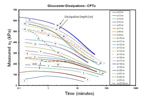
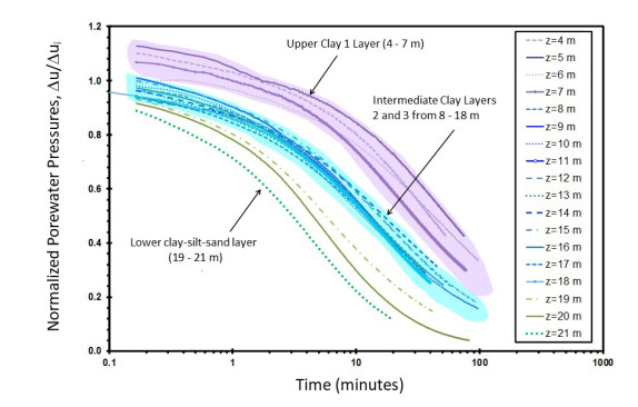
    [13] McQueen W, Miller B, Mayne PW, et al. (2015) Piezocone dissipation tests at the Canadian Test Site No. 1, Gloucester, Ontario. Can Geotech J 53: 884–888.
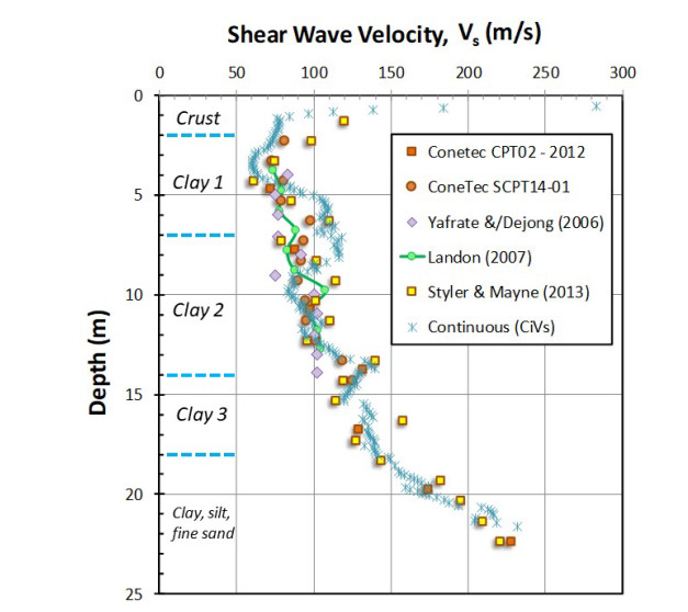
    [14] Styler MA, Mayne PW (2013) Site investigation using continuous shear wave velocity measurements during cone penetration testing at Gloucester, Ontario. Proceedings, GeoMontreal: 66th Canadian Geotechnical Conference, 345.
    [15] Bechai M, Law KT, Craig CBH, et al. (1986) In-situ testing of marine clay for towerline foundations. Proceedings 39th Canadian Geotechnical Conference, Ottawa, 115–122.
    [16] Lutenegger AJ, Timian DA (1986) Flat plate penetrometer tests in marine clays. Proceedings 39th Canadian Geotechnical Conference, Ottawa, 301–309.
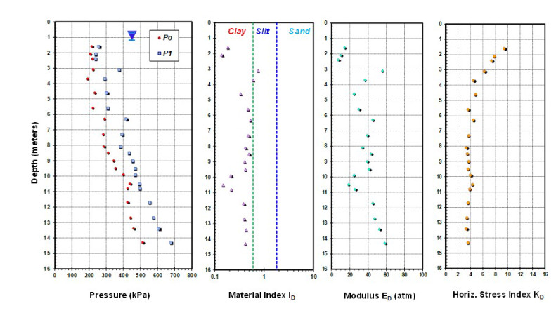
    [17] Lutenegger AJ (2015) Dilatometer tests in sensitive Champlain Sea clay: stress history and shear strength. Proceedings 3rd International Conference on the Flat Dilatometer, Rome.
    [18] Yafrate NJ, DeJong JT (2007) Influence of penetration rate on measured resistance with full flow penetrometers in soft clay. Proceedings GeoDenver, ASCE GSP, Reston, VA.
    [19] Nader A, Fall M, Hache R (2015) Characterization of sensitive marine clays by using cone and ball penetrometers: example of clays in Eastern Canada. Geotech Geol Eng 33: 841–864. doi: 10.1007/s10706-015-9864-x
    [20] Eden WJ, Law KT (1980) Comparison of Undrained shear strength results obtained by different test methods in soft clays. Can Geotech J 17: 369–381. doi: 10.1139/t80-044
    [21] Mayne PW, Peuchen J (2012) Unit weight trends with cone resistance in soft to firm clays. Geotechnical and Geophysical Site Characterization 4 (Proc. ISC-4, Pernambuco), CRC Press, London, 1: 903–910.
    [22] Mayne PW, Peuchen J (2018) Evaluation of CPTU Nkt cone factor for undrained strength of clays. Proceedings 4th International Symposium on Cone Penetration Testing (Technical Univ. Delft), CRC Press/Balkema, 423–430.
    [23] Agaiby SSW (2018) Advancements in the interpretation of seismic piezocone tests in clays and other geomaterials. PhD dissertation, School of Civil & Environmental Engineering, Georgia Institute of Technology, Atlanta, GA: 923.
    [24] Mayne PW, Robertson PK, Lunne T (1998) Clay stress history evaluated from seismic piezocone tests. Geotech Site Charact (Proc. ISC-1, Atlanta), Balkema, Rotterdam, 2: 1113–1118.
    [25] Mayne PW (2007) NCHRP Synthesis 368 on Cone Penetration Test. Transportation Research Board, National Academies Press, Washington, DC, 118.
    [26] Burns SE, Mayne PW (2002) Analytical cavity expansion-critical state model for piezocone dissipation in fine-grained soils. Soils Found 42: 131–137.
    [27] Law KT (1975) Analysis of embankments on sensitive clays. PhD Dissertation, The University of Western Ontario, 521.
    [28] Lo KY, Bozozuk M, Law KT (1976) Settlement analysis of the Gloucester test fill. Can Geotech J 13: 339–354. doi: 10.1139/t76-036
    [29] Hinchberger SD, Rowe RK (1998) Modelling the rate-sensitive characteristics of the Gloucester foundation soil. Can Geotech J 35: 769–789. doi: 10.1139/t98-037
    [30] Radharkrishna HS, Cragg CBH, Tsang R, et al. (1986) Uplift and compression behavior of drilled piers in Leda clay. Proceedings 39th Canadian Geotechnical Conference, Ottawa, 123–130.
    [31] Hosseini MA, Rayhani MT (2015) Evolution of pile shaft capacity over time in soft clays: Case study: Leda clay. Proceedings GeoQuebec: 68th Canadian Geot Conference, Paper ID 793.
    [32] Parez L, Faureil R (1988) Le piézocone. Améliorations apportées ála reconnsaissance de soils. Rev Fr Géotech 44: 13–27.
  • This article has been cited by:

    1. Yang Zhang, Liang Zhao, Jyotindra Narayan, Adaptive control and state error prediction of flexible manipulators using radial basis function neural network and dynamic surface control method, 2025, 20, 1932-6203, e0318601, 10.1371/journal.pone.0318601
  • Reader Comments
  • © 2019 the Author(s), licensee AIMS Press. This is an open access article distributed under the terms of the Creative Commons Attribution License (http://creativecommons.org/licenses/by/4.0)
通讯作者: 陈斌, bchen63@163.com
  • 1. 

    沈阳化工大学材料科学与工程学院 沈阳 110142

  1. 本站搜索
  2. 百度学术搜索
  3. 万方数据库搜索
  4. CNKI搜索

Metrics

Article views(8257) PDF downloads(1901) Cited by(10)

Figures and Tables

Figures(23)

Other Articles By Authors

/

DownLoad:  Full-Size Img  PowerPoint
Return
Return

Catalog