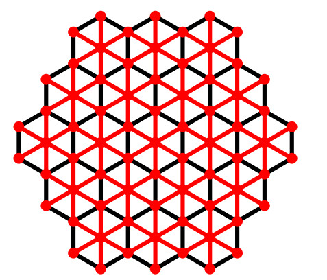
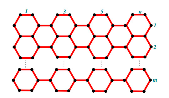
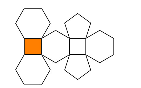
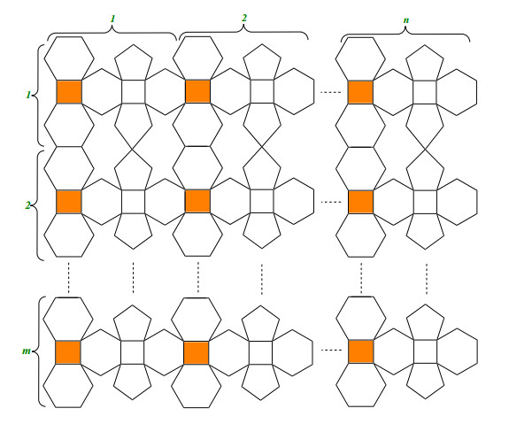
Silicate minerals make up the majority of the earth's crust and account for almost 92 percent of the total. Silicate sheets, often known as silicate networks, are characterised as definite connectivity parallel designs. A key idea in studying different generalised classes of graphs in terms of planarity is the face of the graph. It plays a significant role in the embedding of graphs as well. Face index is a recently created parameter that is based on the data from a graph's faces. The current draft is utilizing a newly established face index, to study different silicate networks. It consists of a generalized chain of silicate, silicate sheet, silicate network, carbon sheet, polyhedron generalized sheet, and also triangular honeycomb network. This study will help to understand the structural properties of chemical networks because the face index is more generalized than vertex degree based topological descriptors.
Citation: Ricai Luo, Khadija Dawood, Muhammad Kamran Jamil, Muhammad Azeem. Some new results on the face index of certain polycyclic chemical networks[J]. Mathematical Biosciences and Engineering, 2023, 20(5): 8031-8048. doi: 10.3934/mbe.2023348
Silicate minerals make up the majority of the earth's crust and account for almost 92 percent of the total. Silicate sheets, often known as silicate networks, are characterised as definite connectivity parallel designs. A key idea in studying different generalised classes of graphs in terms of planarity is the face of the graph. It plays a significant role in the embedding of graphs as well. Face index is a recently created parameter that is based on the data from a graph's faces. The current draft is utilizing a newly established face index, to study different silicate networks. It consists of a generalized chain of silicate, silicate sheet, silicate network, carbon sheet, polyhedron generalized sheet, and also triangular honeycomb network. This study will help to understand the structural properties of chemical networks because the face index is more generalized than vertex degree based topological descriptors.

| [1] |
M. F. Nadeem, M. Azeem, A. Khalil, The locating number of hexagonal möbius ladder network, J. Appl. Math. Comput., 66 (2021), 149–165. https://doi.org/10.1007/s12190-020-01430-8 doi: 10.1007/s12190-020-01430-8

|
| [2] |
A. Ahmad, A. N. Koam, M. Siddiqui, M. Azeem, Resolvability of the starphene structure and applications in electronics, Ain Shams Eng. J., 13 (2022), 101587. https://doi.org/10.1016/j.asej.2021.09.014 doi: 10.1016/j.asej.2021.09.014
|
| [3] |
M. F. Nadeem, M. Imran, H. M. A. Siddiqui, M. Azeem, A. Khalil, Y. Ali, Topological aspects of metal-organic structure with the help of underlying networks, Arab. J. Chem., 14 (2021), 103157. https://doi.org/10.1016/j.arabjc.2021.103157 doi: 10.1016/j.arabjc.2021.103157
|
| [4] | M. Azeem, M. F. Nadeem, Metric-based resolvability of polycyclic aromatic hydrocarbons, Eur. Phys. J. Plus, 136 (2021), 395. |
| [5] |
M. Imran, A. Ahmad, Y. Ahmad, M. Azeem, Edge weight based entropy measure of different shapes of carbon nanotubes, IEEE Access, 9 (2021), 139712–139724. https://doi.org/10.1109/ACCESS.2021.3119032 doi: 10.1109/ACCESS.2021.3119032
|
| [6] |
M. F. Nadeem, A. Shabbir, Computing and comparative analysis of topological invariants of y-junction carbon nanotubes, Int. J. Quant. Chem., 122 (2022), e26847. https://doi.org/10.1002/qua.26847 doi: 10.1002/qua.26847
|
| [7] |
X. Zuo, M. F. Nadeem, M. K. Siddiqui, M. Azeem, Edge weight based entropy of different topologies of carbon nanotubes, IEEE Access, 9 (2021), 102019–102029. https://doi.org/10.1109/ACCESS.2021.3097905 doi: 10.1109/ACCESS.2021.3097905
|
| [8] |
M. F. Nadeem, M. Azeem, H. M. K. Siddiqui, Comparative study of zagreb indices for capped, semi-capped and uncapped carbon nanotubes, Polycyclic Aromat. Compd., 42 (2022), 3545–3562. https://doi.org/10.1080/10406638.2021.1890625 doi: 10.1080/10406638.2021.1890625
|
| [9] |
F. Afzal, S. Hussain, D. Afzal, S. Razaq, Some new degree based topological indices via m-polynomial, J. Inf. Optim. Sci., 41 (2020), 1061–1076. https://doi.org/10.1080/02522667.2020.1744307 doi: 10.1080/02522667.2020.1744307
|
| [10] | A. Rauf, M. Naeem, S. U. Bukhari, Quantitative structure–property relationship of ev-degree and ve-degree based topological indices with physico-chemical properties of benzene derivatives and application, Int. J. Quant. Chem., 122 (2022), e26851. |
| [11] | A. Rauf, M. Naeem, A. Aslam, Quantitative structure–property relationship of edge weighted and degree-based entropy of benzene derivatives, Int. J. Quant. Chem., 122 (2022), e26839. |
| [12] | J. B. Liu, X.-B. Peng, S. Hayat, Topological index analysis of a class of networks analogous to alicyclic hydrocarbons and their derivatives, Int. J. Quant. Chem., 122 (2022), e26827. |
| [13] |
Y. Shang, Sombor index and degree-related properties of simplicial networks, Appl. Math. Comput., 419 (2022), 126881. https://doi.org/10.1016/j.amc.2021.126881 doi: 10.1016/j.amc.2021.126881
|
| [14] |
Z. Wang, Y. Mao, K. C. Das, Y. Shang, Nordhaus–gaddum-type results for the steiner gutman index of graphs, Symmetry, 12 (2020), 1711. https://doi.org/10.3390/sym12101711 doi: 10.3390/sym12101711
|
| [15] |
Y. Shang, Lower bounds for gaussian estrada index of graphs, Symmetry, 10 (2018), 325. https://doi.org/10.3390/sym10080325 doi: 10.3390/sym10080325
|
| [16] |
S. Khan, S. Pirzada, Y. Shang, On the sum and spread of reciprocal distance laplacian eigenvalues of graphs in terms of harary index, Symmetry, 14 (2022), 1937. https://doi.org/10.3390/sym14091937 doi: 10.3390/sym14091937
|
| [17] | J. B. Liu, J. J. Gu, K. Wang, The expected values for the gutman index, schultz index, and some sombor indices of a random cyclooctane chain, Int. J. Quant. Chem., 123 (2022). |
| [18] |
M. Azeem, M. Imran, M. F. Nadeem, Sharp bounds on partition dimension of hexagonal möbius ladder, J. King Saud Univ. Sci., 34 (2022), 101779. https://doi.org/10.1016/j.jksus.2021.101779 doi: 10.1016/j.jksus.2021.101779
|
| [19] |
A. Shabbir, M. Azeem, On the partition dimension of tri-hexagonal alpha-boron nanotube, IEEE Access, 9 (2021), 55644–55653. https://doi.org/10.1109/ACCESS.2021.3071716 doi: 10.1109/ACCESS.2021.3071716
|
| [20] |
J. B. Liu, M. F. Nadeem, M. Azeem, Bounds on the partition dimension of convex polytopes, Comb. Chem. High Throughput Screening, 25 (2022), 547–553. https://doi.org/10.2174/1386207323666201204144422 doi: 10.2174/1386207323666201204144422
|
| [21] | J. B. Liu, Y. Bao, W. T. Zheng, S. Hayat, Network coherence analysis on a family of nested weighted n-polygon networks, Fractals, 29 (2021), 2150260. |
| [22] | J. B. Liu, J. J. Gu, Computing and analyzing the normalized laplacian spectrum and spanning tree of the strong prism of the dicyclobutadieno derivative of linear phenylenes, Int. J. Quant. Chem., 122 (2022), e26972. |
| [23] |
J. B. Liu, J. Zhao, Z. Q. Cai, On the generalized adjacency, laplacian and signless laplacian spectra of the weighted edge corona networks, Phys. A Stat. Mechan. Appl., 540 (2020), 123073. https://doi.org/10.1016/j.physa.2019.123073 doi: 10.1016/j.physa.2019.123073
|
| [24] | J.-B. Liu, J. Zhao, J. Min, J. Cao, The hosoya index of graphs formed by a fractal graph, Fractals, 27 (2019), 1950135. |
| [25] |
J.-B. Liu, C. Wang, S. Wang, and B. Wei, Zagreb indices and multiplicative zagreb indices of eulerian graphs, Bull. Malays. Math. Sci. Soc., 42 (2017), 67–78. https://doi.org/10.1007/s40840-017-0463-2 doi: 10.1007/s40840-017-0463-2
|
| [26] | J. B. Liu, X. F. Pan, Minimizing kirchhoff index among graphs with a given vertex bipartiteness, Appl. Math. Comput., 291 (2016), 84–88. |
| [27] |
J. B. Liu, X. F. Pan, F. T. Hu, F. F. Hu, Asymptotic laplacian-energy-like invariant of lattices, Appl. Math. Comput., 253 (2015), 205–214. https://doi.org/10.1016/j.amc.2014.12.035 doi: 10.1016/j.amc.2014.12.035
|
| [28] |
S. Bukhari, M. K. Jamil, M. Azeem, S. Swaray, Patched network and its vertex-edge metric-based dimension, IEEE Access, 11 (2023), 4478–4485. https://doi.org/10.1109/ACCESS.2023.3235398 doi: 10.1109/ACCESS.2023.3235398
|
| [29] | M. C. Shanmukha, S. Lee, A. Usha, K. C. Shilpa, M. Azeem, Degree-based entropy descriptors of graphenylene using topological indices, Comput. Model. Eng. Sci., 2023 (2023), 1–25. |
| [30] |
X. Zhang, M. T. A. Kanwal, M. Azeem, M. K. Jamil, M. Mukhtar, Finite vertex-based resolvability of supramolecular chain in dialkyltin, Main Group Metal Chem., 45 (2022), 255–264. https://doi.org/10.1515/mgmc-2022-0027 doi: 10.1515/mgmc-2022-0027
|
| [31] |
Q. Huang, A. Khalil, D. A. Ali, A. Ahmad, R. Luo, M. Azeem, Breast cancer chemical structures and their partition resolvability, Math. Biosci. Eng., 20 (2022), 3838–3853. https://doi.org/10.3934/mbe.2023180 doi: 10.3934/mbe.2023180
|
| [32] |
M. Azeem, M. K. Jamil, A. Javed, A. Ahmad, Verification of some topological indices of y-junction based nanostructures by m-polynomials, J. Math., 2022 (2022), 1–18. https://doi.org/10.1155/2022/8238651 doi: 10.1155/2022/8238651
|
| [33] | M. K. Jamil, M. Imran, K. A. Sattar, Novel face index for benzenoid hydrocarbons, Mathematics, 8 (2020), 312. |
| [34] |
X. Zhang, A. Raza, A. Fahad, M. K. Jamil, M. A. Chaudhry, Z. Iqbal, On face index of silicon carbides, Discrete Dyn. Nat. Soc., 2020 (2020), 1–8. https://doi.org/10.1155/2020/6048438 doi: 10.1155/2020/6048438
|
| [35] |
A. Ye, A. Javed, M. K. Jamil, K. A. Sattar, A. Aslam, Z. Iqbal, et al., On computation of face index of certain nanotubes, Discrete Dyn. Nat. Soc., 2020 (2020), 1–6. https://doi.org/10.1155/2020/3468426 doi: 10.1155/2020/3468426
|
| [36] |
Z. Ahmad, , M. Naseem, M. K. Jamil, M. K. Siddiqui, M. F. Nadeem, New results on eccentric connectivity indices of v-phenylenic nanotube, Eurasian Chem. Commun., 2 (2020), 663–671. https://doi.org/10.33945/SAMI/ECC.2020.6.3 doi: 10.33945/SAMI/ECC.2020.6.3
|
| [37] |
Z. Ahmad, , M. Naseem, M. K. Jamil, M. F. Nadeem, S. Wang, Eccentric connectivity indices of titania nanotubes TiO, Eurasian Chem. Commun., 2 (2020), 712–721. https://doi.org/10.33945/SAMI/ECC.2020.6.8 doi: 10.33945/SAMI/ECC.2020.6.8
|
| [38] |
A. N. A. Koam, A. Ahmad, M. Nadeem, Comparative study of valency-based topological descriptor for hexagon star network, Comput. Syst. Sci. Eng., 36 (2021), 293–306. https://doi.org/10.32604/csse.2021.014896 doi: 10.32604/csse.2021.014896
|
| [39] | H. M. A. Siddiqui, S. Baby, M. F. Nadeem, M. K. Shafiq, Bounds of some degree based indices of lexicographic product of some connected graphs, Polycyclic Aromat. Compd., 42 (2022), 2568–2580. |
| [40] |
J. B. Liu, H. M. A. Siddiqui, M. F. Nadeem, M. A. Binyamin, Some topological properties of uniform subdivision of sierpiński graphs, Main Group Metal Chem., 44 (2021), 218–227. https://doi.org/10.1515/mgmc-2021-0006 doi: 10.1515/mgmc-2021-0006
|
| [41] |
M. Ishtiaq, A. Rauf, Q. Rubbab, M. K. Siddiqui, H. Ibrahim, Algebraic polynomial based topological properties of anti-tumor drug hyaluronic acid-doxorubicin (HAD), Polycyclic Aromat. Compd., 42 (2022), 7049–7070. https://doi.org/10.1080/10406638.2021.1995011 doi: 10.1080/10406638.2021.1995011
|
| [42] |
V. Ravi, M. K. Siddiqui, N. Chidambaram, K. Desikan, On topological descriptors and curvilinear regression analysis of antiviral drugs used in COVID-19 treatment, Polycyclic Aromat. Compd., 42 (2022), 6932–6945. https://doi.org/10.1080/10406638.2021.1993941 doi: 10.1080/10406638.2021.1993941
|
| [43] | A. Ahmad, S. C. López, Distance-based topological polynomials associated with zero-divisor graphs, Math. Prob. Eng., 2021 (2021), 1–8. |
| [44] | A. Ahmad, Vertex-degree based eccentric topological descriptors of zero divisor graph of commutative rings, Online J. Anal. Comb., 15 (2020), 1–10. |
| [45] |
A. Ahmad, R. Hasni, K. Elahi, M. A. Asim, Polynomials of degree-based indices for swapped networks modeled by optical transpose interconnection system, IEEE Access, 8 (2020), 214293–214299. https://doi.org/10.1109/ACCESS.2020.3039298 doi: 10.1109/ACCESS.2020.3039298
|
| [46] |
F. A. Abolaban, A. Ahmad, M. A. Asim, Computation of vertex-edge degree based topological descriptors for metal trihalides network, IEEE Access, 9 (2021), 65330–65339. https://doi.org/10.1109/ACCESS.2021.3076036 doi: 10.1109/ACCESS.2021.3076036
|
| [47] |
Özge Çolakoğlu Havare, Topological indices and QSPR modeling of some novel drugs used in the cancer treatment, Int. J. Quant. Chem., 121 (2021), e26813. https://doi.org/10.1002/qua.26813 doi: 10.1002/qua.26813
|
| [48] | J. B. Liu, R. M. Singaraj, Topological analysis of para-line graph of remdesivir used in the prevention of corona virus, Int. J. Quant. Chem., 121 (2021), e26778. |
| [49] | M. M. Zobair, M. A. Malik, H. Shaker, Eccentricity-based topological invariants of tightest nonadjacently configured stable pentagonal structure of carbon nanocones, Int. J. Quant. Chem., 121 (2021), e26807. |
| [50] |
Z. Sabir, M. Umar, M. A. Z. Raja, H. M. Baskonus, W. Gao, Designing of morlet wavelet as a neural network for a novel prevention category in the HIV system, Int. J. Biomath., 15 (2021), 2250012. https://doi.org/10.1142/S1793524522500127 doi: 10.1142/S1793524522500127
|
| [51] |
M. Cancan, D. Afzal, S. Hussain, A. Maqbool, F. Afzal, Some new topological indices of silicate network via m-polynomial, J. Discrete Math. Sci. Cryptography, 23 (2020), 1157–1171. https://doi.org/10.1080/09720529.2020.1809776 doi: 10.1080/09720529.2020.1809776
|
| [52] |
J. B. Liu, M. K. Shafiq, H. Ali, A. Naseem, N. Maryam, S. S. Asghar, Topological indices of mth chain silicate graphs, Mathematics, 7 (2019), 42. https://doi.org/10.3390/math7010042 doi: 10.3390/math7010042
|
| [53] |
A. Q. Baig, M. Imran, H. Ali, On topological indices of poly oxide, poly silicate, DOX, and DSL networks, Can. J. Chem., 93 (2015), 730–739. https://doi.org/10.1139/cjc-2014-0490 doi: 10.1139/cjc-2014-0490
|
| [54] |
M. S. Chen, K. Shin, D. Kandlur, Addressing, routing, and broadcasting in hexagonal mesh multiprocessors, IEEE Trans. Comput., 39 (1990), 10–18. https://doi.org/10.1109/12.46277 doi: 10.1109/12.46277
|
| [55] |
M. F. Nadeem, M. Azeem, I. Farman, Comparative study of topological indices for capped and uncapped carbon nanotubes, Polycyclic Aromat. Compd., 42 (2022), 4666–4683. https://doi.org/10.1080/10406638.2021.1903952 doi: 10.1080/10406638.2021.1903952
|
| [56] |
M. F. Nadeem, M. Azeem, H. M. A. Siddiqui, Comparative study of zagreb indices for capped, semi-capped, and uncapped carbon nanotubes, Polycyclic Aromat. Compd., 42 (2022), 3545–3562. https://doi.org/10.1080/10406638.2021.1890625 doi: 10.1080/10406638.2021.1890625
|
| [57] | M. V. Diudea, C. L. Nagy, Diamond and Related Nanostructures, Springer Netherlands, 2013. https://doi.org/10.1007/978-94-007-6371-5 |
Figures(8) / Tables(5)

Ricai Luo, Khadija Dawood, Muhammad Kamran Jamil, Muhammad Azeem. Some new results on the face index of certain polycyclic chemical networks[J]. Mathematical Biosciences and Engineering, 2023, 20(5): 8031-8048. doi: 10.3934/mbe.2023348


 DownLoad: