


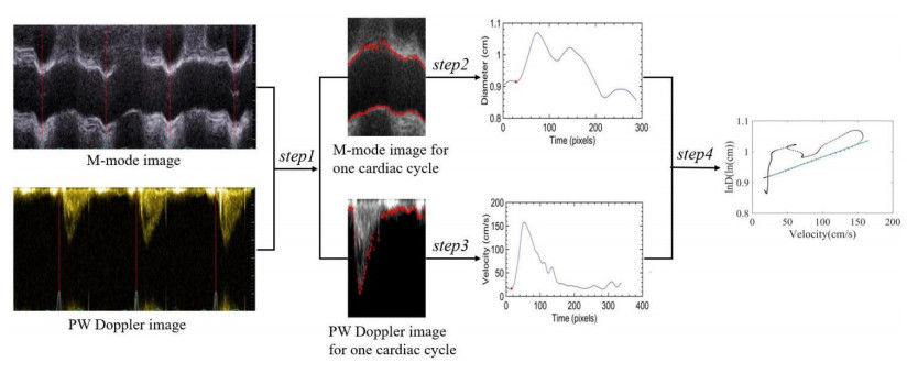
The original diameter velocity loop method (ln(D)U-loop) cannot accurately extract the blood vessel diameter waveform when the quality of ultrasound image data is not high (such as obesity, age, and the operation of the ultrasound doctor), so it is unable to measure the pulse wave velocity (PWV) of the ascending aorta. This study proposes a diameter waveform extraction method combining threshold, gradient filtering, and the center of gravity method. At the same time, the linear regression method of searching for the rising point of the systolic period is replaced by the optimal average of two linear regression methods. This method can also extract the diameter waveform with poor-quality images and obtain a more accurate PWV. In vivo experimental data from 17 (age 60.5 ± 9.2) elderly patients with cerebral infarction and 12 (age 32.5 ± 5.6) healthy young adults were used for processing, and the results showed that the mean PWV using the ln(D)U-loop method was 12.56 (SD = 3.47) ms−1 for patients with cerebral infarction and 6.81 (SD = 1.73) ms−1 for healthy young adults. The PWV results based on the Wilcoxon rank-sum test and calculated based on the improved ln(D)U-loop method were both statistically significant (p < 0.01). The agreement analysis (Bland–Altman analysis) between the QA-loop and ln(D)U-loop methods showed that the mean deviation of the measured PWV was 0.07 m/s and the standard deviation of the deviation was 1.18 m/s. The experimental results demonstrated the effectiveness of the improved ln(D)U-loop method proposed in this paper on poor-quality images. This study can improve the possibility of the ln(D)U-loop method being widely used in the clinical measurement of ascending aortic PWV.
Citation: Shuyan Liu, Peilin Li, Yuanhao Tan, Geqi Ding, Bo Peng. A robust local pulse wave imaging method based on digital image processing techniques[J]. Mathematical Biosciences and Engineering, 2023, 20(4): 6721-6734. doi: 10.3934/mbe.2023289
| [1] | Zhongzi Zhao, Meng Yan . Positive radial solutions for the problem with Minkowski-curvature operator on an exterior domain. AIMS Mathematics, 2023, 8(9): 20654-20664. doi: 10.3934/math.20231052 |
| [2] | Wenjia Li, Guanglan Wang, Guoliang Li . The local boundary estimate of weak solutions to fractional p-Laplace equations. AIMS Mathematics, 2025, 10(4): 8002-8021. doi: 10.3934/math.2025367 |
| [3] | Sobajima Motohiro, Wakasugi Yuta . Remarks on an elliptic problem arising in weighted energy estimates for wave equations with space-dependent damping term in an exterior domain. AIMS Mathematics, 2017, 2(1): 1-15. doi: 10.3934/Math.2017.1.1 |
| [4] | Limin Guo, Jiafa Xu, Donal O'Regan . Positive radial solutions for a boundary value problem associated to a system of elliptic equations with semipositone nonlinearities. AIMS Mathematics, 2023, 8(1): 1072-1089. doi: 10.3934/math.2023053 |
| [5] | Keqiang Li, Shangjiu Wang . Symmetry of positive solutions of a p-Laplace equation with convex nonlinearites. AIMS Mathematics, 2023, 8(6): 13425-13431. doi: 10.3934/math.2023680 |
| [6] | Zhanbing Bai, Wen Lian, Yongfang Wei, Sujing Sun . Solvability for some fourth order two-point boundary value problems. AIMS Mathematics, 2020, 5(5): 4983-4994. doi: 10.3934/math.2020319 |
| [7] | Lin Zhao . Monotonicity and symmetry of positive solution for 1-Laplace equation. AIMS Mathematics, 2021, 6(6): 6255-6277. doi: 10.3934/math.2021367 |
| [8] | Manal Alfulaij, Mohamed Jleli, Bessem Samet . A hyperbolic polyharmonic system in an exterior domain. AIMS Mathematics, 2025, 10(2): 2634-2651. doi: 10.3934/math.2025123 |
| [9] | Maria Alessandra Ragusa, Abdolrahman Razani, Farzaneh Safari . Existence of positive radial solutions for a problem involving the weighted Heisenberg p(⋅)-Laplacian operator. AIMS Mathematics, 2023, 8(1): 404-422. doi: 10.3934/math.2023019 |
| [10] | Zhiqian He, Liangying Miao . Multiplicity of positive radial solutions for systems with mean curvature operator in Minkowski space. AIMS Mathematics, 2021, 6(6): 6171-6179. doi: 10.3934/math.2021362 |
The original diameter velocity loop method (ln(D)U-loop) cannot accurately extract the blood vessel diameter waveform when the quality of ultrasound image data is not high (such as obesity, age, and the operation of the ultrasound doctor), so it is unable to measure the pulse wave velocity (PWV) of the ascending aorta. This study proposes a diameter waveform extraction method combining threshold, gradient filtering, and the center of gravity method. At the same time, the linear regression method of searching for the rising point of the systolic period is replaced by the optimal average of two linear regression methods. This method can also extract the diameter waveform with poor-quality images and obtain a more accurate PWV. In vivo experimental data from 17 (age 60.5 ± 9.2) elderly patients with cerebral infarction and 12 (age 32.5 ± 5.6) healthy young adults were used for processing, and the results showed that the mean PWV using the ln(D)U-loop method was 12.56 (SD = 3.47) ms−1 for patients with cerebral infarction and 6.81 (SD = 1.73) ms−1 for healthy young adults. The PWV results based on the Wilcoxon rank-sum test and calculated based on the improved ln(D)U-loop method were both statistically significant (p < 0.01). The agreement analysis (Bland–Altman analysis) between the QA-loop and ln(D)U-loop methods showed that the mean deviation of the measured PWV was 0.07 m/s and the standard deviation of the deviation was 1.18 m/s. The experimental results demonstrated the effectiveness of the improved ln(D)U-loop method proposed in this paper on poor-quality images. This study can improve the possibility of the ln(D)U-loop method being widely used in the clinical measurement of ascending aortic PWV.
Boundary value problems with p-Laplace operator Δpu=div(|∇u|p−2∇u) arise in many different areas of applied mathematics and physics, such as non-Newtonian fluids, reaction-diffusion problems, non-linear elasticity, etc. But little is known about the p-Laplace operator cases (p≠2) compared to the vast amount of knowledge for the Laplace operator (p=2). In this paper, we discuss the existence of positive radial solution for the p-Laplace boundary value problem (BVP)
| {−Δpu=K(|x|)f(u),x∈Ω,∂u∂n=0,x∈∂Ω,lim|x|→∞u(x)=0, | (1.1) |
in the exterior domain Ω={x∈RN:|x|>r0}, where N≥2, r0>0, 1<p<N, ∂u∂n is the outward normal derivative of u on ∂Ω, K:[r0,∞)→R+ is a coefficient function, f:R+→R is a nonlinear function. Throughout this paper, we assume that the following conditions hold:
(A1) K∈C([r0,∞),R+) and 0<∫∞r0rN−1K(r)dr<∞;
(A2) f∈C(R+,R+);
For the special case of p=2, namely the Laplace boundary value problem
| {−Δu=K(|x|)f(u),x∈Ω,∂u∂n=0,x∈∂Ω,lim|x|→∞u(x)=0, | (1.2) |
the existence of positive radial solutions has been discussed by many authors, see [1,2,3,4,5,6,7]. The authors of references[1,2,3,4,5,6] obtained some existence results by using upper and lower solutions method, priori estimates technique and fixed point index theory. In [7], the present author built an eigenvalue criteria of existing positive radial solutions. The eigenvalue criterion is related to the principle eigenvalue λ1 of the corresponding radially symmetric Laplace eigenvalue problem (EVP)
| {−Δu=λK(|x|)u,x∈Ω,∂u∂n=0,x∈∂Ω,u=u(|x|),lim|x|→∞u(|x|)=0. | (1.3) |
Specifically, if f satisfies one of the following eigenvalue conditions:
(H1) f0<λ1, f∞>λ1;
(H2) f∞<λ1, f0>λ1,
the BVP(1.2) has a classical positive radial solution, where
| f0=lim infu→0+f(u)u,f0=lim supu→0+f(u)u,f∞=lim infu→∞f(u)u,f∞=lim supu→∞f(u)u. |
See [7,Theorem 1.1]. This criterion first appeared in a boundary value problem of second-order ordinary differential equations, and built by Zhaoli Liu and Fuyi Li in [8]. Then it was extended to general boundary value problems of ordinary differential equations, See [9,10]. In [11,12], the radially symmetric solutions of the more general Hessian equations are discussed.
The purpose of this paper is to establish a similar existence result of positive radial solution of BVP (1.1). Our results are related to the principle eigenvalue λp,1 of the radially symmetric p-Laplce eigenvalue problem (EVP)
| {−Δpu=λK(|x|)|u|p−2u,x∈Ω,∂u∂n=0,x∈∂Ω,u=u(|x|),lim|x|→∞u(|x|)=0. | (1.4) |
Different from EVP (1.3), EVP (1.4) is a nonlinear eigenvalue problem, and the spectral theory of linear operators is not applicable to it. In Section 2 we will prove that EVP (1.4) has a minimum positive real eigenvalue λp,1, see Lemma 2.3. For BVP (1.1), we conjecture that eigenvalue criteria is valid if f0, f0, f∞ and f∞ is replaced respectively by
| fp0=lim infu→0+f(u)up−1,fp0=lim supu→0+f(u)up−1,fp∞=lim infu→∞f(u)up−1,fp∞=lim supu→∞f(u)up−1. | (1.5) |
But now we can only prove a weaker version of it: In second inequality of (H1) and (H2), λp,1 needs to be replaced by the larger number
| B=[∫10Ψ(∫1stp−1a(t)dt)ds]−(p−1), | (1.6) |
where a∈C+(0,1] is given by (2.4) and Ψ∈C(R) is given by (2.7). Our result is as follows:
Theorem 1.1. Suppose that Assumptions (A1) and (A2) hold. If the nonlinear function f satisfies one of the the following conditions:
(H1)∗ fp0<λp,1, fp∞>B;
(H2)∗ fp∞<λp,1, fp0>B,
then BVP (1.1) has at least one classical positive radial solution.
As an example of the application of Theorem 1.1, we consider the following p-Laplace boundary value problem
| {−Δpu=K(|x|)|u|γ,x∈Ω,∂u∂n=0,x∈∂Ω,lim|x|→∞u(x)=0. | (1.7) |
Corresponding to BVP (1.1), f(u)=|u|γ. If γ>p−1, by (1.5) fp0=0, fp∞=+∞, and (H1) holds. If 0<γ<p−1, then fp∞=0, fp0=+∞, and (H2) holds. Hence, by Theorem 1.1 we have
Corollary 1. Let K:[r0,∞)→R+ satisfy Assumption (A1), γ>0 and γ≠p−1. Then BVP (1.7) has a positive radial solution.
The proof of Theorem 1.1 is based on the fixed point index theory in cones, which will be given in Section 3. Some preliminaries to discuss BVP (1.1) are presented in Section 2.
For the radially symmetric solution u=u(|x|) of BVP (1.1), setting r=|x|, since
| −Δpu=div(|∇u|p−2∇u)=−(|u′(r)|p−2u′(r))′−N−1r|u′(r)|p−2u′(r), |
BVP (1.1) becomes the ordinary differential equation BVP in [r0,∞)
| {−(|u′(r)|p−2u′(r))′−N−1r|u′(r)|p−2u′(r)=K(r)f(u(r)),r∈[r0,∞),u′(r0)=0,u(∞)=0, | (2.1) |
where u(∞)=limr→∞u(r).
Let q>1 be the constant satisfying 1p+1q=1. To solve BVP (2.1), make the variable transformations
| t=(r0r)(q−1)(N−p),r=r0t−1/(q−1)(N−p),v(t)=u(r(t)), | (2.2) |
Then BVP (2.1) is converted to the ordinary differential equation BVP in (0,1]
| {−(|v′(t)|p−2v′(t))′=a(t)f(v(t)),t∈(0,1],v(0)=0,v′(1)=0, | (2.3) |
where
| a(t)=rq(N−1)(t)(q−1)p(N−p)pr0q(N−p)K(r(t)),t∈(0,1]. | (2.4) |
BVP (2.3) is a quasilinear ordinary differential equation boundary value problem with singularity at t=0. A solution v of BVP (2.3) means that v∈C1[0,1] such that |v′|p−2v′∈C1(0,1] and it satisfies the Eq (2.3). Clearly, if v is a solution of BVP (2.3), then u(r)=v(t(r)) is a solution of BVP (2.1) and u(|x|) is a classical radial solution of BVP (1.1). We discuss BVP (2.3) to obtain positive radial solutions of BVP (1.1).
Let I=[0,1] and R+=[0,+∞). Let C(I) denote the Banach space of all continuous function v(t) on I with norm ‖v‖C=maxt∈I|v(t)|, C1(I) denote the Banach space of all continuous differentiable function on I. Let C+(I) be the cone of all nonnegative functions in C(I).
To discuss BVP (2.3), we first consider the corresponding simple boundary value problem
| {−(|v′(t)|p−2v′(t))′=a(t)h(t),t∈(0,1],v(0)=0,v′(1)=0, | (2.5) |
where h∈C+(I) is a given function. Let
| Φ(v)=|v|p−2v=|v|p−1sgnv,v∈R, | (2.6) |
then w=Φ(v) is a strictly monotone increasing continuous function on R and its inverse function
| Φ−1(w):=Ψ(w)=|w|q−1sgnw,w∈R, | (2.7) |
is also a strictly monotone increasing continuous function.
Lemma 2.1. For every h∈C(I), BVP (2.5) has a unique solution v:=Sh∈C1(I). Moreover, the solution operator S:C(I)→C(I) is completely continuous and has the homogeneity
| S(νh)=νq−1Sh,h∈C(I),ν≥0. | (2.8) |
Proof. By (2.4) and Assumption (A1), the coefficient a(t)∈C+(0,1] and satisfies
| ∫10a(t)dt=1[(q−1)(N−p)]p−1r0N−p∫∞r0rN−1K(r)dr<∞. | (2.9) |
Hence a∈L(I).
For every h∈C(I), we verify that
| v(t)=∫t0Ψ(∫1sa(τ)h(τ)dτ)ds:=Sh(t),t∈I | (2.10) |
is a unique solution of BVP (2.5). Since the function G(s):=∫1sa(τ)h(τ)dτ∈C(I), from (2.10) it follows that v∈C1(I) and
| v′(t)=Ψ(∫1ta(τ)h(τ)dτ),t∈I. | (2.11) |
Hence,
| |v′(t)|p−2v′(t)=Φ(v′(t))=∫1ta(τ)h(τ)dτ,t∈I. |
This means that (|v′(t)|p−2v′(t)∈C1(0,1] and
| (|v′(t)|p−2v′(t))′=−a(t)h(t),t∈(0,1], |
that is, v is a solution of BVP (2.5).
Conversely, if v is a solution of BVP (2.5), by the definition of the solution of BVP (2.5), it is easy to show that v can be expressed by (2.10). Hence, BVP (2.5) has a unique solution v=Sh.
By (2.10) and the continuity of Ψ, the solution operator S:C(I)→C(I) is continuous. Let D⊂C(I) be bounded. By (2.10) and (2.11) we can show that S(D) and its derivative set {v′|v∈S(D)} are bounded sets in C(I). By the Ascoli-Arzéla theorem, S(D) is a precompact subset of C(I). Thus, S:C(I)→C(I) is completely continuous.
By the uniqueness of solution of BVP (2.5), we easily verify that the solution operator S satisfies (2.8).
Lemma 2.2. If h∈C+(I), then the solution v=Sh of LBVP (2.5) satisfies: ‖v‖c=v(1), v(t)≥t‖v‖C for every t∈I.
Proof. Let h∈C+(I) and v=Sh. By (2.10) and (2.11), for every t∈I v(t)≥0 and v′(t)≥0. Hence, v(t) is a nonnegative monotone increasing function and ‖v‖C=maxt∈Iv(t)=v(1). From (2.11) and the monotonicity of Ψ, we notice that v′(t) is a monotone decreasing function on I. For every t∈(0,1), by Lagrange's mean value theorem, there exist ξ1∈(0,t) and ξ2∈(t,1), such that
| (1−t)v(t)=(1−t)(v(t)−v(0))=v′(ξ1)t(1−t)≥v′(t)t(1−t),tv(t)=tv(1)−t(v(1)−v(t))=tv(1)−tv′(ξ2)(1−t)≥tv(1)−v′(t)t(1−t). |
Hence
| v(t)=tv(t)+(1−t)v(t)≥tv(1)=t‖v‖C. |
Obviously, when t=0 or 1, this inequality also holds. The proof is completed.
Consider the radially symmetric p-Laplace eigenvalue problem EVP (1.3). We have
Lemma 2.3. EVP (1.4) has a minimum positive real eigenvalue λp,1, and λp,1 has a radially symmetric positive eigenfunction.
Proof. For the radially symmetric eigenvalue problem EVP (1.4), writing r=|x| and making the variable transformations of (2.2), it is converted to the one-dimensional weighted p-Laplace eigenvalue problem (EVP)
| {−(|v′(t)|p−2v′(t))′=λa(t)|v(t)|p−2v(t),t∈(0,1],v(0)=0,v′(1)=0, | (2.12) |
where v(t)=u(r(t)). Clearly, λ∈R is an eigenvalue of EVP (1.4) if and only if it is an eigenvalue of EVP (2.12). By (2.4) and (2.9), a∈C+(0,1]∩L(I) and ∫10a(s)ds>0. This guarantees that EVP (2.12) has a minimum positive real eigenvalue λp,1, which given by
| λp,1=inf{∫10|w′(t)|pdt∫10a(t)wp(t)dt|w∈C1(I),w(0)=0,w′(1)=0,∫10a(t)wp(t)dt≠0}. | (2.13) |
Moreover, λp,1 is simple and has a positive eigenfunction ϕ∈C+(I)∩C1(I). See [13, Theorem 5], [14, Theorem 1.1] or [15, Theorem 1.2]. Hence, λp,1 is also the minimum positive real eigenvalue of EVP (1.4), and ϕ((r0/|x|)(q−1)(N−p)) is corresponding positive eigenfunction.
Now we consider BVP (2.3). Define a closed convex cone K of C(I) by
| K={v∈C(I)|v(t)≥t‖v‖C,t∈I}. | (2.14) |
By Lemma 2.2, S(C+(I))⊂K. Let f∈C(R+,R+), and define a mapping F:K→C+(I) by
| F(v)(t):=f(v(t)),t∈I. | (2.15) |
Then F:K→C+(I) is continuous and it maps every bounded subset of K into a bounded subset of C+(I). Define the composite mapping by
| A=S∘F. | (2.16) |
Then A:K→K is completely continuous by the complete continuity of the operator S:C+(I)→K. By the definitions of S and K, the positive solution of BVP (2.3) is equivalent to the nonzero fixed point of A.
Let E be a Banach space and K⊂E be a closed convex cone in E. Assume D is a bounded open subset of E with boundary ∂D, and K∩D≠∅. Let A:K∩¯D→K be a completely continuous mapping. If Av≠v for every v∈K∩∂D, then the fixed point index i(A,K∩D,K) is well defined. One important fact is that if i(A,K∩D,K)≠0, then A has a fixed point in K∩D. In next section, we will use the following two lemmas in [16,17] to find the nonzero fixed point of the mapping A defined by (2.16).
Lemma 2.4. Let D be a bounded open subset of E with 0∈D, and A:K∩¯D→K a completely continuous mapping. If μAv≠v for every v∈K∩∂D and 0<μ≤1, then i(A,K∩D,K)=1.
Lemma 2.5. Let D be a bounded open subset of E with 0∈D, and A:K∩¯D→K a completely continuous mapping. If ‖Av‖≥‖v‖ and Av≠v for every v∈K∩∂D, then i(A,K∩D,K)=0.
Proof of Theorem 1.1. We only consider the case that (H1)* holds, and the case that (H2)* holds can be proved by a similar way.
Let K⊂C(I) be the closed convex cone defined by (2.14) and A:K→K be the completely continuous mapping defined by (2.16). If v∈K is a nontrivial fixed point of A, then by the definitions of S and A, v(t) is a positive solution of BVP (2.3) and u=v(r0N−2/|x|N−2) is a classical positive radial solution of BVP (1.1). Let 0<R1<R2<+∞ and set
| D1={v∈C(I):‖v‖C<R1},D2={v∈C(I):‖v‖C<R2}. | (3.1) |
We prove that A has a fixed point in K∩(¯D2∖D1) when R1 is small enough and R2 large enough.
Since fp0<λp,1, by the definition of fp0, there exist ε∈(0,λp,1) and δ>0, such that
| f(u)≤(λp,1−ε)up−1,0≤u≤δ. | (3.2) |
Choosing R1∈(0,δ), we prove that A satisfies the condition of Lemma 2.4 in K∩∂D1, namely
| μAv≠v,∀v∈K∩∂D1,0<μ≤1. | (3.3) |
In fact, if (3.3) does not hold, there exist v0∈K∩∂D1 and 0<μ0≤1 such that μ0Av0=v0. By the homogeneity of S, v0=μ0S(F(v0))=S(μ0p−1F(v0)). By the definition of S, v0 is the unique solution of BVP (2.5) for h=μ0p−1F(v0)∈C+(I). Hence, v0∈C1(I) satisfies the differential equation
| {−(|v′0(t)|p−2v0′(t))′=μ0p−1a(t)f(v0(t)),t∈(0,1],v0(0)=0,v0′(1)=0. | (3.4) |
Since v0∈K∩∂D1, by the definitions of K and D1,
| 0≤v0(t)≤‖v0‖C=R1<δ,t∈I. |
Hence by (3.2),
| f(v0(t))≤(λp,1−ε)v0p−1(t),t∈I. |
By this inequality and Eq (3.4), we have
| −(|v′0(t)|p−2v0′(t))′≤μ0p−1(λp,1−ε)a(t)v0p−1(t),t∈(0,1]. |
Multiplying this inequality by v0(t) and integrating on (0,1], then using integration by parts for the left side, we have
| ∫10|v′0(t)|pdt≤μ0p−1(λp,1−ε)∫10a(t)v0p(t)dt≤(λp,1−ε)∫10a(t)v0p(t)dt. | (3.5) |
Since v0∈K∩∂D, by the definition of K,
| ∫10a(t)v0p(t)dt≥‖v0‖Cp∫10tpa(t)dt=R1p∫10tpa(t)dt>0. |
Hence, by (2.13) and (3.5) we obtain that
| λp,1≤∫10|v′0(t)|pdt∫10a(t)v0p(t)dt≤λp,1−ε, |
which is a contradiction. This means that (3.3) holds, namely A satisfies the condition of Lemma 2.4 in K∩∂D1. By Lemma 2.4, we have
| i(A,K∩D1,K)=1. | (3.6) |
On the other hand, by the definition (1.6) of B, we have
| B<[∫1σΨ(∫1stp−1a(t)dt)ds]−(p−1)→B(σ→0+),σ∈(0,1). | (3.7) |
Since fp∞>B, by (3.7) there exists σ0∈(0,1), such that
| B0:=[∫1σ0Ψ(∫1stp−1a(t)dt)ds]−(p−1)<fp∞. | (3.8) |
By this inequality and the definition of fp∞, there exists H>0 such that
| f(u)>B0up−1,u>H. | (3.9) |
Choosing R2>max{δ,H/σ0}, we show that
| ‖Av‖C≥‖v‖C,v∈K∩∂D2. | (3.10) |
For ∀v∈K∩∂D2 and t∈[σ0,1], by the definitions of K and D2
| v(t)≥t‖v‖C≥σ0R2>H. |
By this inequality and (3.9),
| f(v(t))>B0vp−1(t)≥B0‖v‖p−1Ctp−1,t∈[σ0,1]. | (3.11) |
Since Av=S(F(v)), by the expression (2.10) of the solution operator S and (3.11), noticing (p−1)(q−1)=1, we have
| ‖Av‖C≥Av(1)=∫10Ψ(∫1sa(t)f(v(t))dt)ds≥∫1σ0Ψ(∫1sa(t)f(v(t))dt)ds≥∫1σ0Ψ(∫1sa(t)B0‖v‖p−1Ctp−1dt)ds=Bq−10‖v‖C∫1σ0Ψ(∫1stp−1a(t)dt)ds=‖v‖C. |
Namely, (3.10) holds. Suppose A has no fixed point on ∂D2. Then by (3.10), A satisfies the condition of Lemma 2.5 in K∩∂D2. By Lemma 2.5, we have
| i(A,K∩D2,K)=0. | (3.12) |
By the additivity of fixed point index, (3.6) and (3.11), we have
| i(A,K∩(D2∖¯D1),K)=i(A,K∩D2,K)−i(A,K∩D1,K)=−1. |
Hence A has a fixed point in K∩(D2∖¯D1).
The proof of Theorem 1.1 is complete.
The authors would like to express sincere thanks to the reviewers for their helpful comments and suggestions. This research was supported by National Natural Science Foundations of China (No.12061062, 11661071).
The authors declare that they have no competing interests.
| [1] |
M. Ezzati, Z. Obermeyer, I. Tzoulaki, B. M. Mayosi, P. Elliott, D. A. Leon, Contributions of risk factors and medical care to cardiovascular mortality trends, Nat. Rev. Cardiol., 12 (2015), 508–530. https://doi.org/10.1038/nrcardio.2015.82 doi: 10.1038/nrcardio.2015.82

|
| [2] | L. Y. Ma, W. W. Chen, R. L. Gao, L. S. Liu, M. L. Zhu, Y. J. Wang, et al., China cardiovascular diseases report 2018: An updated summary, J. Geriatr Cardiol., 17 (2020), 1–8. |
| [3] |
T. Pereira, C. Correia, J. Cardoso, Novel methods for pulse wave velocity measurement, J. Med. Biol. Eng., 35 (2015), 555–565. https://doi.org/10.1007/s40846-015-0086-8. doi: 10.1007/s40846-015-0086-8
|
| [4] | S. Zhang, L. Sun, H. Ju, Z. Bao, X. A. Zeng, S. Lin, Research advances and application of pulsed electric field on proteins and peptides in food, Food Res. Int., 139 (2021), 109914. |
| [5] |
S. Laurent, J. Cockcroft, L. Van Bortel, P. Boutouyrie, C. Giannattasio, D. Hayoz, et al., Expert consensus document on arterial stiffness: Methodological issues and clinical applications, Eur. Heart J., 27 (2006), 2588–2605. https://doi.org/10.1093/eurheartj/ehl254 doi: 10.1093/eurheartj/ehl254
|
| [6] |
B. Li, H. Gao, X. Li, Y. Liu, M. Wang, Correlation between Brachial-Ankle pulse wave velocity and arterial compliance and cardiovascular risk factors in elderly patients with arteriosclerosis, Hypertens. Res., 29 (2006), 309–314. https://doi.org/10.1291/hypres.29.309 doi: 10.1291/hypres.29.309
|
| [7] | H. L. Kim, S. H. Kim, Pulse wave velocity in atherosclerosis, Front. Cardiovasc. Med., 6 (2019), 41. |
| [8] | A. Jeevarethinam, S. Venuraju, A. Dumo, S. Ruano, V. S. Mehta, M. Rosenthal, et al., Relationship between carotid atherosclerosis and coronary artery calcification in asymptomatic diabetic patients: A prospective multicenter study, Clin. Cardiol., 40 (2017), 752–758. |
| [9] | W. Yang, Y. Wang, Y. Yu, L. Mu, F. Kong, J. Yang, et al., Establishing normal reference value of carotid ultrafast pulse wave velocity and evaluating changes on coronary slow flow, Int. J. Cardiovasc. Imaging, 36 (2020), 1931–1939. |
| [10] | A. Pribadi, T. A. T. Nasution, H. Zakaria, T. L. R. Mengko, Brachial-Ankle pulse wave velocity calculation methods based on oscillometric pressure measurement for arterial stiffness assessment, in 2018 2nd International Conference on Biomedical Engineering (IBIOMED), (2018), 1–6. https://doi.org/10.1109/IBIOMED.2018.8534778 |
| [11] |
Y. Li, C. Wang, M. Zhao, S. Yao, M. Wang, S. Zhang, et al., Effect of brachial-ankle pulse wave velocity combined with waist-to-hip ratio on cardiac and cerebrovascular events, Am. J. Med. Sci., 362 (2021), 135–142. https://doi.org/10.1016/j.amjms.2021.02.014 doi: 10.1016/j.amjms.2021.02.014
|
| [12] |
N. Piko, S. Bevc, R. Hojs, F. H. Naji, R. Ekart, The association between pulse wave analysis, carotid-femoral pulse wave velocity and peripheral arterial disease in patients with ischemic heart disease, BMC Cardiovasc. Disord., 21 (2021), 33. https://doi.org/10.1186/s12872-021-01859-0 doi: 10.1186/s12872-021-01859-0
|
| [13] | K. V. Raj, P. M. Nabeel, J. Joseph, Image-Free fast ultrasound for measurement of local pulse wave velocity: In vitro validation and in vivo feasibility, IEEE Trans. Ultrason. Ferroelectr. Freq. Control., 69 (2022), 2248–2256. |
| [14] |
J. Liu, K. Wang, H. Liu, H. Zhao, W. Huang, N. Zhao, et al., Cross-Sectional relationship between carotid-femoral pulse wave velocity and biomarkers in vascular-related diseases, Int. J. Hypertens., 2020 (2020), 6578731. https://doi.org/10.1155/2020/6578731 doi: 10.1155/2020/6578731
|
| [15] |
H. Ji, J. Xiong, S. Yu, C. Chi, B. Bai, J. Teliewubai, et al., Measuring the carotid to femoral pulse wave velocity (Cf-PWV) to evaluate arterial stiffness, Medicine, (2018). https://doi.org/10.3791/57083 doi: 10.3791/57083
|
| [16] |
C. J. Tang, P. Y. Lee, Y. H. Chuang, C. C. Huang, Measurement of local pulse wave velocity for carotid artery by using an ultrasound-based method, Ultrasonics, 102 (2020), 106064. https://doi.org/10.1016/j.ultras.2020.106064 doi: 10.1016/j.ultras.2020.106064
|
| [17] |
A. Tentolouris, I. Eleftheriadou, P. Grigoropoulou, A. Kokkinos, G. Siasos, I. Ntanasis-Stathopoulos, et al., The association between pulse wave velocity and peripheral neuropathy in patients with type 2 diabetes mellitus, J. Diabetes Its Complications, 31 (2017), 1624–1629. https://doi.org/10.1016/j.jdiacomp.2017.07.010 doi: 10.1016/j.jdiacomp.2017.07.010
|
| [18] |
X. Liu, J. Liu, X. Xu, L. Chun, J. Tang, Y. Deng, A robust detail preserving anisotropic diffusion for speckle reduction in ultrasound images, BMC Genomics, 12 (2011), S14. https://doi.org/10.1186/1471-2164-12-S5-S14 doi: 10.1186/1471-2164-12-S5-S14
|
| [19] |
J. Tang, S. Guo, Q. Sun, Y. Deng, D. Zhou, Speckle reducing bilateral filter for cattle follicle segmentation, BMC Genomics, 11 (2010), S9. https://doi.org/10.1186/1471-2164-11-S2-S9 doi: 10.1186/1471-2164-11-S2-S9
|
| [20] |
J. Luo, R. X. Li, E. E. Konofagou, Pulse wave imaging of the human carotid artery: An in vivo feasibility study, IEEE Trans. Ultrason. Ferroelectr. Freq. Control., 59 (2012), 174–181. https://doi.org/10.1109/TUFFC.2012.2170 doi: 10.1109/TUFFC.2012.2170
|
| [21] |
C. Huang, T. L. Ren, J. Luo, Effects of parameters on the accuracy and precision of ultrasound-based local pulse wave velocity measurement: A simulation study, IEEE Trans. Ultrason. Ferroelectr. Freq. Control., 61 (2014), 2001–2018. https://doi.org/10.1109/TUFFC.2014.006597 doi: 10.1109/TUFFC.2014.006597
|
| [22] |
G. Fiori, F. Fuiano, A. Scorza, S. Conforto, S. A. Sciuto, Non-Invasive methods for PWV measurement in blood vessel stiffness assessment, IEEE Rev. Biomed. Eng., 15 (2022), 169–183. https://doi.org/10.1109/RBME.2021.3092208 doi: 10.1109/RBME.2021.3092208
|
| [23] | M. Negoita, A. D. Hughes, K. H. Parker, A. W. Khir, Non-invasive technique for determining local pulse wave velocity in humans ascending aorta, Comput. Cardiol., 1–4. https://doi.org/10.22489/CinC.2017.218-036 |
| [24] |
M. Negoita, A. D. Hughes, K. H. Parker, A. W. Khir, A method for determining local pulse wave velocity in human ascending aorta from sequential ultrasound measurements of diameter and velocity, Physiol. Meas., 39 (2018), 114009. https://doi.org/10.1088/1361-6579/aae8a0 doi: 10.1088/1361-6579/aae8a0
|
| [25] |
S. I. Rabben, N. Stergiopulos, L. R. Hellevik, O. A. Smiseth, S. Slørdahl, S. Urheim, et al., An ultrasound-based method for determining pulse wave velocity in superficial arteries, J. Biomech., 37 (2004), 1615–1622. https://doi.org/10.1016/j.jbiomech.2003.12.031 doi: 10.1016/j.jbiomech.2003.12.031
|
| [26] | J. Feng, A. W. Khir, Determination of wave speed and wave separation in the arteries using diameter and velocity, J. Biomech., 43 (2010), 455–462. |
| [27] | H. Qun, Using linear array CCD for long distance diffraction alignment measurment, Opt. Technol., (1999). |
| [28] |
A. A. Tijsseling, A. W. Anderson, Johannes von Kries and the History of Water Hammer, J. Hydraul. Eng., 133 (2007), 1–8. https://doi.org/10.1061/(ASCE)0733-9429(2007)133:1(1) doi: 10.1061/(ASCE)0733-9429(2007)133:1(1)
|
| [29] |
J. R. Womersley, Method for the calculation of velocity, rate of flow and viscous drag in arteries when the pressure gradient is known, J. Phys., 127 (1955), 553–563. https://doi.org/10.1113/jphysiol.1955.sp005276 doi: 10.1113/jphysiol.1955.sp005276
|
| [30] |
D. W. Holdsworth, C. J. Norley, R. Frayne, D. A. Steinman, B. K. Rutt, Characterization of common carotid artery blood-flow waveforms in normal human subjects, Phys. Meas., 20 (1999), 219–240. https://doi.org/10.1088/0967-3334/20/3/301 doi: 10.1088/0967-3334/20/3/301
|
| 1. | Bo Yang, Radially Symmetric Positive Solutions of the Dirichlet Problem for the p-Laplace Equation, 2024, 12, 2227-7390, 2351, 10.3390/math12152351 | |
| 2. | Yongxiang Li, Pengbo Li, Radial solutions of p-Laplace equations with nonlinear gradient terms on exterior domains, 2023, 2023, 1029-242X, 10.1186/s13660-023-03069-y | |
| 3. | 旭莹 唐, The Existence of Positive Solutions to Quasilinear Differential Equation on Infinite Intervals, 2023, 13, 2160-7583, 2103, 10.12677/PM.2023.137217 |


Figures(8) / Tables(1)

Shuyan Liu, Peilin Li, Yuanhao Tan, Geqi Ding, Bo Peng. A robust local pulse wave imaging method based on digital image processing techniques[J]. Mathematical Biosciences and Engineering, 2023, 20(4): 6721-6734. doi: 10.3934/mbe.2023289


 DownLoad: