External intervention model with direct and indirect propagation behaviors on social media platforms

Fulian Yin; Xinyi Tang; Tongyu Liang; Yanjing Huang; Jianhong Wu; Fulian Yin; Xinyi Tang; Tongyu Liang; Yanjing Huang; Jianhong Wu

doi:10.3934/mbe.2022530

Mathematical Biosciences and Engineering

2022, Volume 19, Issue 11: 11380-11398. doi: 10.3934/mbe.2022530

Previous Article Next Article

Research article

External intervention model with direct and indirect propagation behaviors on social media platforms

1.
State Key Laboratory of Media Convergence and Communication, Communication University of China, Beijing 100024, China
2.
College of Information and Communication Engineering, Communication University of China, Beijing 100024, China
3.
Fields-CQAM Laboratory of Mathematics for Public Health, Laboratory for Industrial and Applied Mathematics, York University, Toronto M3J1P3, Canada

Academic Editor: Zi-Gang Huang

Received: 10 May 2022 Revised: 21 July 2022 Accepted: 26 July 2022 Published: 09 August 2022

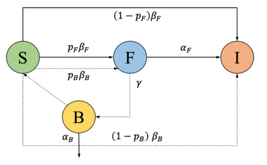
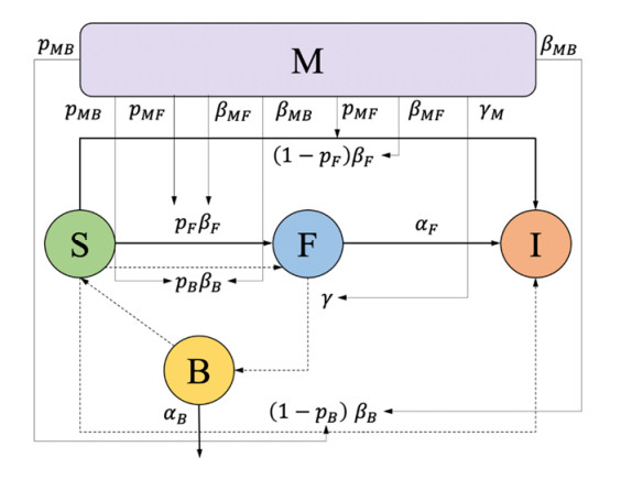
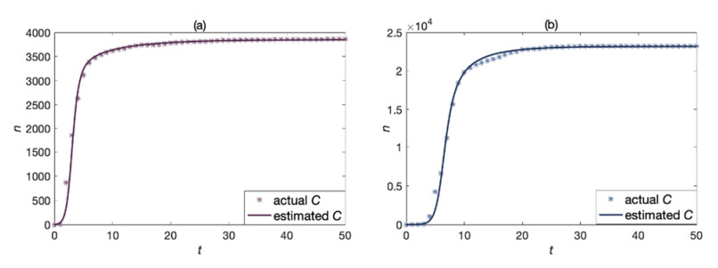
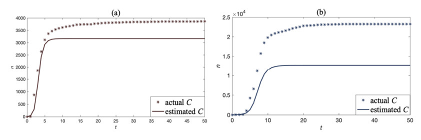
A significant distinction between the COVID-19 pandemic and previous pandemics is the significant role of social media platforms in shaping public adherence to non-pharmaceutical interventions and vaccine acceptance. However, with the recurrence of the epidemic, the conflict between epidemic prevention and production recovery has become increasingly prominent on social media. To help design effective communication strategies to guide public opinion, we propose a susceptible-forwarding-immune pseudo-environment (SFI-PE) dynamic model for understanding the environment with direct and indirect propagation behaviors. Then, we introduce a system with external interventions for direct and indirect propagation behaviors, termed the macro-controlled SFI-PE (M-SFI-PE) model. Based on the numerical analyses that were performed using actual data from the Chinese Sina microblogging platform, the data fitting results prove our models' effectiveness. The research grasps the law of the new information propagation paradigm, and our work bridges the gap between reality and theory in information interventions.

Keywords:

Citation: Fulian Yin, Xinyi Tang, Tongyu Liang, Yanjing Huang, Jianhong Wu. External intervention model with direct and indirect propagation behaviors on social media platforms[J]. Mathematical Biosciences and Engineering, 2022, 19(11): 11380-11398. doi: 10.3934/mbe.2022530

Related Papers:

[1]	M. Hafiz Uddin, M. Ali Akbar, Md. Ashrafuzzaman Khan, Md. Abdul Haque . New exact solitary wave solutions to the space-time fractional differential equations with conformable derivative. AIMS Mathematics, 2019, 4(2): 199-214. doi: 10.3934/math.2019.2.199
[2]	Gulnur Yel, Haci Mehmet Baskonus, Wei Gao . New dark-bright soliton in the shallow water wave model. AIMS Mathematics, 2020, 5(4): 4027-4044. doi: 10.3934/math.2020259
[3]	Chander Bhan, Ravi Karwasra, Sandeep Malik, Sachin Kumar, Ahmed H. Arnous, Nehad Ali Shah, Jae Dong Chung . Bifurcation, chaotic behavior and soliton solutions to the KP-BBM equation through new Kudryashov and generalized Arnous methods. AIMS Mathematics, 2024, 9(4): 8749-8767. doi: 10.3934/math.2024424
[4]	Khudhayr A. Rashedi, Saima Noor, Tariq S. Alshammari, Imran Khan . Lump and kink soliton phenomena of Vakhnenko equation. AIMS Mathematics, 2024, 9(8): 21079-21093. doi: 10.3934/math.20241024
[5]	F. A. Mohammed . Soliton solutions for some nonlinear models in mathematical physics via conservation laws. AIMS Mathematics, 2022, 7(8): 15075-15093. doi: 10.3934/math.2022826
[6]	Ye Zhao, Chunfeng Xing . Orbital stability of periodic traveling waves to some coupled BBM equations. AIMS Mathematics, 2023, 8(9): 22225-22236. doi: 10.3934/math.20231133
[7]	Miao Yang, Lizhen Wang . Lie symmetry group, exact solutions and conservation laws for multi-term time fractional differential equations. AIMS Mathematics, 2023, 8(12): 30038-30058. doi: 10.3934/math.20231536
[8]	M. Mossa Al-Sawalha, Humaira Yasmin, Ali M. Mahnashi . Kink phenomena of the time-space fractional Oskolkov equation. AIMS Mathematics, 2024, 9(11): 31163-31179. doi: 10.3934/math.20241502
[9]	Nauman Raza, Maria Luz Gandarias, Ghada Ali Basendwah . Symmetry reductions and conservation laws of a modified-mixed KdV equation: exploring new interaction solutions. AIMS Mathematics, 2024, 9(4): 10289-10303. doi: 10.3934/math.2024503
[10]	Abdelkader Moumen, Khaled A. Aldwoah, Muntasir Suhail, Alwaleed Kamel, Hicham Saber, Manel Hleili, Sayed Saifullah . Investigation of more solitary waves solutions of the stochastics Benjamin-Bona-Mahony equation under beta operator. AIMS Mathematics, 2024, 9(10): 27403-27417. doi: 10.3934/math.20241331

Abstract

1. Introduction

Nonlinear partial differential equations (NPDEs) are crucial due to their ability to decode a wide-ranging of phenomena, as well as wave bending, fluid mechanics, hydrodynamics, organic molecular dispersion, magnetism, thermal conductivity, and many more. These phenomena are found across multiple scientific areas, such as mathematics, physics, engineering, biology, and finance. The broad range of NLPDEs is shown by a variety of equations, such as the Higgs system, advection equation, Boussinesq equation, Fisher's equation, and Burger's equation, among others ^[1,2,3,4,5].

Several asymptotic methods have been proposed in other studies to explore the internal dynamic behaviors of nonlinear partial differential equations (NPDEs) and fractional NPDEs with investigations on propagating solitons and other travelling wave solutions ^[6,7,8,9,10]. A soliton is an auto-oscillating wave-packet that preserves both its shape and speed during its propagation due to the fine-tuning between dispersion and nonlinearity. Kink waves, shock waves, lump waves, damped waves, periodic waves, etc are a few examples of solitons are present, which are described by soliton theory ^[11,12,13]. Despite the abundant availability of numerical solutions, analysts often resort to analytical methods because of the ability to explain the flow of physics and the accuracy of estimate of the behaviors of the system ^[14,15,16]. As a result, work on developing analytical treatments to investigate the solitonic behavior of NPDEs and fractional NPDEs is still ongoing, and several analytical methods have been created to investigate soliton solutions. $F$ -expansion technique ^[17], sech-tanh technique ^[18], Sardar sub-equation technique ^[19], $(G'/G)$ -expansion technique ^{[20,21,22,23]}, exp-function technique ^[24], sub-equation technique ^[25], tanh technique ^[26], $(G'/G^2)$ -expansion technique ^[27], Hirota bilinear technique ^[28], Kudryashov technique ^[29], Poincaré-Lighthill Kuo approach ^[30], unified technique ^[31], Riccati-Bernoulli Sub-ODE technique ^[32], extended direct algebraic technique ^{[33,34,35,36,37]}, auxiliary equation method ^[38], simple equation method ^[39], and RMESEM ^[40] are a few of these methods.

To discover cases of propagating solitons and other traveling waves, results for NPDEs and NFPDEs, this work establishes a new modification in a novel analytical technique called RMESEM with extended Riccati equation. This approach uses a variable-form wave transformation to transform the NPDE or NFPDE into an integer-order NODE. The resulting NODE is considered to have a series-based result (incorporating the solution of the Riccati equation). The substitution of the supposed solution in the resultant NODE transforms it into a set of algebraic equations. The soliton solutions for the relevant NPDEs and NFPDEs are acquired by more thoroughly finding the solutions of algebraic equations. The families of soliton solutions produced by RMESEM with the extended Riccati equation can help us comprehend the fundamental physical mechanisms and behavioral patterns of the nonlinear system.

To showcase the effectiveness of the improved RMESEM, the method is utilized to acquire soliton solutions for the (2+1)-dimensional GZK-BBME. In 1972, Benjamin et al. ^[41] investigated the issue of long waves with small and finite amplitudes and put out the Benjamin-Bona-Mahony equation (BBME), which took the following form:

$\begin{equation} v_t+\alpha v_x+\beta v v_x-\gamma v_{txx} = 0. \end{equation}$

(1.1)

To study weakly nonlinear ion-acoustic oscillations in low-pressure magnetized plasma, Zakharov and Kuznetsov ^[42] extended the Korteweg-de Vries (KdV) equation, resulting in the formulation of the Zakharov-Kuznetsov equation (ZKE) as:

$\begin{equation} v_t+\alpha v v_x+(v_{xx}+v_{yy}+v_{zz})_x = 0, \end{equation}$

(1.2)

where $v$ denotes ion velocity with the magnetic fields and is non-dimensional. Wazwaz ^[43] merged the ZKE and BBME equations in 2005 to create the (2+1) dimensional GZK-BBM equation ^[40]:

$\begin{equation} v_t+v_x+\alpha (v^\delta)_x+\beta(v_{xt}+v_{yy})_x = 0, \quad \delta > 1, \end{equation}$

(1.3)

where $v = v(t, x, y)$ , the coefficients $\alpha$ and $\beta$ are the relative dispersion and nonlinear parameters respectively, and $x$ and $y$ are the propagating & transverse coordinates. The nonlinear influence is introduced into the equation by the term $(v^\delta)_x$ . This formula is applied to the ZK-model analysis of long waves with finite amplitude. This equation's odd-order derivatives, $v_{xxt}$ and $v_{yyx}$ , take the dispersion effect into account. Examining the way the nonlinear and dispersion effects interact with the problem is one goal of the generalized GZK-BBME investigation. For instance, the tanh and sine-cosine approach was used to solve (3) ^[44]. By using a modified simple equation approach, Khan et al. ^[45] were able to get solitary wave solutions to the GZK-BBME for $n = 3$ . In 2015, Guner et al. ^[46] revealed the dark and bright soliton solution of the GZK-BBME. Finally, Patel and Kumar acquired numerical and semi-analytical solutions for GZK-BBME for $n = 2$ and $n = 3$ by the Adomian decomposition method and the variational iteration method, respectively, under some initial conditions ^[40]. The remaining task of the present analysis is to constructs and examine the propagation of the solitons in the context of GZK-BBME for $n = 3$ articulated in (2.1).

The rest of the study is structured as follows: In Section 2, we detail the working process of RMESEM. Following this approach, we develop soliton solutions for the GZK-BBME in Section 3. The depictions and graphical discussion are presented in Section 4. Lastly, Section 5 provides the conclusion in our research proposal.

2. The operational methodology of RMESEM

This section outlines the operational mechanism of RMESEM for constructing soliton solutions for NPDEs. Suppose the following general NPDE:

$\begin{equation} P( v , v_t, v_{x}, v_{y}, v v_{t}, \ldots) = 0, \end{equation}$

(2.1)

where $v = v(t, x, y)$ is an unknown function, $P$ is the polynomial of $v(t, x, y)$ , while the subscripts signify partial derivatives.

The main steps of the proposed RMESEM are as follows:

Step 1. Take into consideration the ensuing wave transformation

$\begin{equation} v(t, x, y) = V(\zeta), \quad \text{where} \quad \zeta = x+y- \omega t, \end{equation}$

(2.2)

where $\omega$ denotes wave speed. Equation (2.1) is converted into the following NODE using the above wave transformation:

$\begin{equation} Q(V, V'V, V', \dots) = 0, \end{equation}$

(2.3)

where the primes indicate the ordinary derivatives of $V$ with respect to $\zeta$ , and $Q$ is a polynomial of $V$ and its derivatives.

Step 2. Equation (2.3) is sometimes integrated term by term to be made conformable for the homogeneous balancing rule.

Step 3. Following that, we suppose that a closed-form wave solution for Eq (2.3) can be expressed in the ensuing form:

$\begin{equation} V(\zeta) = \sum\limits_{j = 0}^{\gamma}k_j \left(\frac{\Phi'(\zeta)}{\Phi(\zeta)}\right)^j+ \sum\limits_{\epsilon = 0}^{\gamma-1}s_\epsilon \left(\frac{\Phi'(\zeta)}{\Phi(\zeta)}\right)^\epsilon \cdot \left(\frac{1}{\Phi(\zeta)} \right), \end{equation}$

(2.4)

where $k_j (j = 0, ..., \gamma)$ and $s_\epsilon (\epsilon = 0, ..., \gamma-1)$ represent the unknown constants that need to be determined later and $\Phi(\zeta)$ satisfies the subsequent 1st order Riccati equation:

$\begin{equation} \Phi'(\zeta) = p+q \Phi(\zeta)+r(\Phi(\zeta))^2, \end{equation}$

(2.5)

where $p, q$ and $r$ are constants.

Step 4. To calculate the integer $\gamma$ presented in Eq (2.4), we take the homogeneous balance between the highest nonlinear term and the highest-order derivative term in Eq (2.3).

Step 5. Substituting the value of $\gamma$ got in step 4 into Eq (2.4) and substituting the result together with $\Phi(\zeta)$ raised to the exponent equal to the index of the integral on the left-hand side of Eq (2.3) or substituting the result with $\Phi(\zeta)$ when we have integrated Eq (2.3) gives an expression in terms of $\Phi(\zeta)$ . New additional construction by comparison of coefficient expression gives a system of algebraic equations of $k_j (j = 0, ..., \gamma)$ and $s_\epsilon (\epsilon = 0, ..., \gamma-1)$ with other associated parameters that are introduced.

Step 6. Solving the algebraic system obtained in Step 5 with the help of algebraic software Maple yields values of $k_j (j = 0, ..., \gamma)$ and $s_\epsilon (\epsilon = 0, ..., \gamma-1)$ with additional associated parameters.

Step 7. Finally, soliton solutions to Eq (2.1) are derived by determining and substituting the calculated values of parameters in Eq (2.4) with the solutions of Eq (2.5) that are given in Table 1.

Table 1. The solutions

$\Phi(\zeta)$ that meet the particular Riccati equation in (2.4) and the structure of

$\bigg(\frac{\Phi'(\zeta)}{\Phi(\zeta)}\bigg)$ , where

$\kappa = q^2-4r p$ and

$\wp = \cosh \left(\frac{1}{4}\, \sqrt {\kappa}\zeta \right) \sinh \left(\frac{1}{4}\, \sqrt {\kappa}\zeta \right)$ .

S. No.	Family	Condition(s)	$\Phi(\zeta)$	$\bigg(\frac{\Phi'(\zeta)}{\Phi(\zeta)}\bigg)$
1	Trigonometric Solutions	$\kappa < 0, \quad r\neq0$
	Trigonometric Solutions		$-{\frac {q}{2r}}+{\frac {\sqrt {-\kappa}\tan \left(\frac{1}{2}\, \sqrt {-\kappa}\zeta \right) }{2r}}$ ,	$-\frac{1}{2}\, {\frac {\kappa\, \left(1+ \left(\tan \left(\frac{1}{2}\, \sqrt {-\kappa}\zeta \right) \right) ^{2} \right) }{-q+\sqrt {-\kappa}\tan \left(\frac{1}{2}\, \sqrt {-\kappa}\zeta \right) }}$ ,
			$-{\frac {q}{2r}}-{\frac {\sqrt {-\kappa}\cot \left(\frac{1}{2}\, \sqrt {-\kappa}\zeta \right) }{2r}}$ ,	$\frac{1}{2}\, {\frac { \left(1+ \left(\cot \left(\frac{1}{2}\, \sqrt {-\kappa}\zeta \right) \right) ^{2} \right) \kappa}{q+\sqrt {-\kappa}\cot \left(\frac{1}{2}\, \sqrt {-\kappa}\zeta \right) }}$ ,
			$-{\frac {q}{2r}}+{\frac {\sqrt {-\kappa} \left(\tan \left(\sqrt{-\kappa}\zeta \right) + \left(\sec \left(\sqrt {-\kappa}\zeta \right) \right) \right) }{2r}}$ ,	$-{\frac {\kappa\, \left(1+\sin \left(\sqrt {-\kappa}\zeta \right) \right) \sec \left(\sqrt {-\kappa}\zeta \right)}{ -q\cos \left(\sqrt {-\kappa}\zeta \right) +\sqrt {-\kappa}\sin \left(\sqrt {-\kappa}\zeta \right) +\sqrt {-\kappa} }}$ ,
			$-{\frac {q}{2r}}+{\frac {\sqrt {-\kappa} \left(\tan \left(\sqrt{-\kappa}\zeta \right) - \left(\sec \left(\sqrt {-\kappa}\zeta \right) \right) \right) }{2r}}$ .	${\frac {\kappa\, \left(\sin \left(\sqrt {-\kappa}\zeta \right) -1 \right) \sec \left(\sqrt {-\kappa}\zeta \right)}{ -q\cos \left(\sqrt {-\kappa}\zeta \right) +\sqrt {-\kappa}\sin \left(\sqrt {-\kappa}\zeta \right) -\sqrt {-\kappa} }}$ .
2	Rational Solutions
	Rational Solutions	$\kappa=0$	$-2\, {\frac {p \left(q\zeta\, +2 \right) }{{q}^{2}\zeta\, }}$ ,	$-2\, {\frac {1}{\zeta\, \left(q\zeta+2 \right) }}$ ,
		$\kappa=0$ , & $q=r=0$	$\zeta\, p$ ,	$\frac {1}{\zeta\, }$ ,
		$\kappa=0$ , & $q=p=0$	$-{\frac {1}{\zeta\, r}}$ .	$-\frac {1}{\zeta\, }$ .
3	Hyperbolic Solutions	$\kappa > 0, \quad r\neq0$
	Hyperbolic Solutions		$-{\frac {q}{2r}}-{\frac {\sqrt {\kappa}\tanh \left(\frac{1}{2}\, \sqrt {\kappa}\zeta \right) }{2r}}$ ,	$-\frac{1}{2}\, {\frac { \left(-1+ \left(\tanh \left(\frac{1}{2}\, \sqrt {\kappa}\zeta \right) \right) ^{2} \right) \kappa}{q+\sqrt {\kappa}\tanh \left(\frac{1}{2}\, \sqrt {\kappa}\zeta \right) }}$ ,
			$-{\frac {q}{2r}}-{\frac {\sqrt {\kappa} \left(\tanh \left(\sqrt{\kappa}\zeta \right) + i \left({\rm sech} \left(\sqrt {\kappa}\zeta \right) \right) \right) }{2r}}$ ,	$-{\frac {\kappa\, \left(-1+i\sinh \left(\sqrt {\kappa}\zeta \right) \right) }{\cosh \left(\sqrt {\kappa}\zeta \right) \left(q\cosh \left(\sqrt {\kappa}\zeta \right) +\sqrt {\kappa}\sinh \left(\sqrt { \kappa}\zeta \right) +i\sqrt {\kappa} \right) }}$ ,
			$-{\frac {q}{2r}}-{\frac {\sqrt {\kappa} \left(\tanh \left(\sqrt{\kappa}\zeta \right) - i \left({\rm sech} \left(\sqrt {\kappa}\zeta \right) \right) \right) }{2r}}$ ,	$-{\frac {\kappa\, \left(1+i\sinh \left(\sqrt {\kappa}\zeta \right) \right) }{\cosh \left(\sqrt {\kappa}\zeta \right) \left(-q\cosh \left(\sqrt {\kappa}\zeta \right) -\sqrt {\kappa}\sinh \left(\sqrt { \kappa}\zeta \right) +i\sqrt {\kappa} \right) }},$
			$-{\frac {q}{2r}}-{\frac {\sqrt {\kappa} \left(\coth \left(\sqrt{\kappa}\zeta \right) + \left({\rm csch} \left(\sqrt {\kappa}\zeta \right) \right) \right) }{2r}}$ .	$-\frac{1}{4}\, {\frac {\kappa\, \left(2\, \left(\cosh \left(\frac{1}{4}\, \sqrt { \kappa}\zeta \right) \right) ^{2}-1 \right) }{\wp \left(-2\, q\wp +\sqrt {\kappa} \right) }}.$
4	Rational-Hyperbolic Solutions
		$p=0$ , & $q\neq0$ , $r\neq 0$	$-{\frac {\lambda\, b}{r \left(\cosh \left(b \zeta \right) -\sinh \left(b \zeta \right) +\lambda \right) }}$ ,	${\frac {q \left(\sinh \left(q\zeta \right) -\cosh \left(q\zeta \right) \right) }{-\cosh \left(q\zeta \right) +\sinh \left(q\zeta \right) -\lambda}}$ ,
			$-{\frac {b \left(\cosh \left(b \zeta \right) +\sinh \left(b \zeta \right) \right) }{r \left(\cosh \left(b \zeta \right) +\sinh \left(b \zeta \right) +\mu \right) }}$ .	${\frac {q\mu}{\cosh \left(q\zeta \right) +\sinh \left(q\zeta \right) + \mu}}$ .
5	Exponential Solutions
	Exponential Solutions	$r=0$ , & $q=\Upsilon$ , $p=h\Upsilon$	${e}^{\Upsilon\, \zeta}-h$ ,	${\frac {\Upsilon\, {{\rm e}^{\Upsilon\, \zeta}}}{{{\rm e}^{\Upsilon\, \zeta}}-h}}$ ,
		$p=0$ , & $q=\Upsilon$ , $r=h\Upsilon$	${\frac {{e}^{\Upsilon\, \zeta}}{1-h{e}^{\Upsilon \zeta}}}$ .	$-{\frac {\Upsilon}{-1+h{{\rm e}^{\Upsilon\, \zeta}}}}$ .

| Show Table

DownLoad: CSV

3. Execution of RMESEM

This section employs the proposed RMESEM for the establishment of new plethora of soliton solutions for GZK-BBME with $\delta = 3$ of the form:

$\begin{equation} v_t+v_x+\alpha (v^3)_x+\beta(v_{xt}+v_{yy})_x = 0. \end{equation}$

(3.1)

We proceed by performing the wave transformation given in Eq (2.2), which transforms Eq (3.1) into the ensuing NODE:

$\begin{equation} -\omega V'+V'+\alpha (V^3)'+\beta(-\omega V''+V'')' = 0. \end{equation}$

(3.2)

Upon integrating Eq (3.2) with zero constant of integration, we obtain the following NODE:

$\begin{equation} (1-\omega) V+\alpha V^3+ (1-\omega) \beta V''. \end{equation}$

(3.3)

Establishing the principle of homogenous balance between terms $V''$ and $V^3$ in Eq (3.3) suggests that $2 +\gamma = 3 \gamma$ which applies $\gamma = 1$ . Substituting $\gamma = 1$ in Eq (2.4) presents the series form closed solutions for Eq (3.3):

$\begin{equation} V(\zeta) = \sum\limits_{j = 0}^{1}k_j \left(\frac{\Phi'(\zeta)}{\Phi(\zeta)}\right)^j+ \left(\frac{s_0 }{\Phi(\zeta)} \right). \end{equation}$

(3.4)

An expression in $\Phi(\zeta)$ is generated by entering Eq (3.4) into Eq (3.3) and gathering all terms with the equal exponents of $\Phi(\zeta)$ . The achieved expressions can be reduced to the ensuing scheme of seven nonlinear algebraic equations by putting the coefficients to zero:

$\begin{equation*} \begin{split} 2\, \beta\, k_{{1}}{r}^{3}-2\, \beta\, \omega\, k_{{1}}{r}^{3}+\alpha\, {k_{{1} }}^{3}{r}^{3} = 0, \end{split} \end{equation*}$

$\begin{equation*} \begin{split} 3\, \alpha\, {k_{{1}}}^{3}q{r}^{2}-3\, \beta\, \omega\, k_{{1}}q{r}^{2}+3\, \alpha\, k_{{0}}{k_{{1}}}^{2}{r}^{2}+3\, \beta\, k_{{1}}q{r}^{2} = 0, \end{split} \end{equation*}$

$\begin{equation*} \begin{split} & -2\, \beta\, \omega\, k_{{1}}{r}^{2}p+2\, \beta\, k_{{1}}{r}^{ 2}p+3\, \alpha\, {k_{{0}}}^{2}k_{{1}}r-\beta\, \omega\, k_{{1}}{q}^{2}r+3\, \alpha\, {k_{{1}}}^{3}p{r}^{2}\\ &-\omega\, k_{{1}}r+k_{{1}}r+3\, \alpha\, {k_{{1}}}^{3}{q}^{ 2}r+6\, \alpha\, k_{{0}}{k_{{1}}}^{2}qr+\beta\, k_{{1}}{q}^{2}r+3\, \alpha \, {k_{{1}}}^{2}{r}^{2}s_{{0}} = 0, \end{split} \end{equation*}$

$\begin{equation*} \begin{split} & 6\, \alpha\, {k_{{1}}}^{3}pqr+\alpha\, {k_{{0}}}^{3}+2\, \beta\, k_{{1}}qpr +6\, \alpha\, k_{{0}}k_{{1}}rs_{{0}}+k_{{1}}q-\omega\, k_{{1}}q+6\, \alpha\, k_{{0}}{k_{{1}}}^{2}pr+3\, \alpha\, {k_{{0}}}^{2}k_{{1}}q\\ &+6\, \alpha\, {k_{{1}}}^{2}qrs_{{0}}+k_{{0}}+\beta\, s_{{0}}qr-\beta\, \omega\, s_ {{0}}qr+\alpha\, {k_{{1}}}^{3}{q}^{3}+3\, \alpha\, k_{{0}}{k_{{1}}}^{2} {q}^{2}-\omega\, k_{{0}}-2\, \beta\, \omega\, k_{{1}}qpr = 0, \end{split} \end{equation*}$

$\begin{equation*} \begin{split} & -\omega\, s_{{0}}+\beta\, s_{{0}}{q}^{2}+6\, \alpha\, {k_{{1}}}^{2}prs_{{0} }+6\, \alpha\, k_{{0}}{k_{{1}}}^{2}pq+3\, \alpha\, {k_{{1}}}^{3}{p}^{2}r -\omega\, k_{{1}}p+k_{{1}}p+3\, \alpha\, {k_{{0}}}^{2}s_{{0}}\\ &-2\, \beta\, \omega\, k_{{1}}r{p}^{2}+s_{{0}}-2\, \beta\, \omega\, s_{{0}}pr+6\, \alpha\, k_{{0}}k_{{1}}qs_{{0}}+3\, \alpha\, {k_{{0}}}^{2}k_{{1}}p+2\, \beta\, s_{{0 }}pr+\beta\, k_{{1}}{q}^{2}p\\ &+3\, \alpha\, k_{{1}}r{s_{{0}}}^{2}+3\, \alpha \, {k_{{1}}}^{3}p{q}^{2}-\beta\, \omega\, s_{{0}}{q}^{2}+3\, \alpha\, {k_{{1 }}}^{2}{q}^{2}s_{{0}}+2\, \beta\, k_{{1}}r{p}^{2}-\beta\, \omega\, k_{{1}}{q}^ {2}p = 0, \end{split} \end{equation*}$

$\begin{equation*} \begin{split} & 3\, \alpha\, {k_{{1}}}^{3}{p}^{2}q+3\, \beta\, s_{{0}}pq+3\, \alpha\, k_{{1} }q{s_{{0}}}^{2}-3\, \beta\, \omega\, s_{{0}}pq+6\, \alpha\, k_{{0}}k_{{1}}ps _{{0}}\\ &-3\, \beta\, \omega\, k_{{1}}q{p}^{2}+6\, \alpha\, {k_{{1}}}^{2}pqs_{{0 }}+3\, \alpha\, k_{{0}}{k_{{1}}}^{2}{p}^{2}+3\, \beta\, k_{{1}}q{p}^{2}+3\, \alpha\, k_{{0}}{s_{{0}}}^{2} = 0, \end{split} \end{equation*}$

and

$\begin{equation*} \begin{split} -2\, \beta\, \omega\, s_{{0}}{p}^{2}+\alpha\, {k_{{1}}}^{3}{p}^{3}+3\, \alpha\, {k_{{1}}}^{2}{p}^{2}s_{{0}}+\alpha\, {s_{{0}}}^{3}-2\, \beta\, \omega\, k_{{1}}{p}^{3}+2\, \beta\, s_{{0}}{p}^{2}+3\, \alpha\, k_{{1}}p{s_{ {0}}}^{2}+2\, \beta\, k_{{1}}{p}^{3} = 0. \end{split} \end{equation*}$

When tackling the result scheme with Maple, the followings three sorts of results become available:

Case 1.

$\begin{equation} \begin{split} k_{{1}} = 0, \; \; s_{{0}} = s_{{0}}, \; \; k_{{0}} = \frac{1}{2}\, {\frac {s_{{0}}q}{p}}, \; \; \beta = \frac{2\, }{ \kappa}, \; \; \alpha = 4\, {\frac {{p}^{2} \left( \omega-1 \right) }{ \kappa\, {s_{{0}}}^{2}}}, \; \; \omega = \omega. \end{split} \end{equation}$

(3.5)

Case 2.

$\begin{equation} \begin{split} k_{{1}} = k_{{1}}, \; \; s_{{0}} = s_{{0}}, \; \; k_{{0}} = k_{{0}}, \; \; \beta = \beta, \; \; \alpha = 0, \; \; \omega = 1. \end{split} \end{equation}$

(3.6)

Case 3.

$\begin{equation} \begin{split} k_{{1}} = k_{{1}}, \; \; s_{{0}} = -k_{{1}}p, \; \; k_{{0}} = -\frac{1}{2}\, k_{{1}}q, \; \; \beta = \frac{2\, }{ \kappa}, \; \; \alpha = 4\, {\frac {\omega-1}{\kappa\, {k_{{1}}}^{2}}}, \; \; \omega = \omega. \end{split} \end{equation}$

(3.7)

When Case 1 is assumed and Eqs (2.2) and (3.4), together with the consistent general result of Eq (2.5) given in Table 1. The following cases of soliton results for GZK-BBME expressed in Eq (3.1) result:

Set. 1.1. With $\kappa < 0, \; r\neq0$ ,

$\begin{equation} \begin{split} v_{1, 1}(x, y, t) = \frac{1}{2}\, {\frac {s_{{0}}q}{p}}+s_{{0}} \left( -\frac{1}{2}\, {\frac {q}{r}}+\frac{1}{2}\, { \frac {\sqrt {-\kappa}\tan \left( \frac{1}{2}\, \sqrt {-\kappa}\zeta \right) }{r }} \right) ^{-1} , \end{split} \end{equation}$

(3.8)

$\begin{equation} \begin{split} v_{1, 2}(x, y, t) = \frac{1}{2}\, {\frac {s_{{0}}q}{p}}+s_{{0}} \left( -\frac{1}{2}\, {\frac {q}{r}}-\frac{1}{2}\, { \frac {\sqrt {-\kappa}\cot \left( \frac{1}{2}\, \sqrt {-\kappa}\zeta \right) }{r }} \right) ^{-1} , \end{split} \end{equation}$

(3.9)

$\begin{equation} \begin{split} v_{1, 3}(x, y, t) = \frac{1}{2}\, {\frac {s_{{0}}q}{p}}+s_{{0}} \left( -\frac{1}{2}\, {\frac {q}{r}}+\frac{1}{2}\, { \frac {\sqrt {-\kappa} \left( \tan \left( \sqrt {-\kappa}\zeta \right) +\sec \left( \sqrt {-\kappa}\zeta \right) \right) }{r}} \right) ^{-1} , \end{split} \end{equation}$

(3.10)

and

$\begin{equation} \begin{split} v_{1, 4}(x, y, t) = \frac{1}{2}\, {\frac {s_{{0}}q}{p}}+s_{{0}} \left( -\frac{1}{2}\, {\frac {q}{r}}+\frac{1}{2}\, { \frac {\sqrt {-\kappa} \left( \tan \left( \sqrt {-\kappa}\zeta \right) -\sec \left( \sqrt {-\kappa}\zeta \right) \right) }{r}} \right) ^{-1} . \end{split} \end{equation}$

(3.11)

Set. 1.2. With $\kappa > 0, \; r\neq0$ ,

$\begin{equation} \begin{split} v_{1, 5}(x, y, t) = \frac{1}{2}\, {\frac {s_{{0}}q}{p}}+s_{{0}} \left( -\frac{1}{2}\, {\frac {q}{r}}-\frac{1}{2}\, { \frac {\sqrt {\kappa}\tanh \left( \frac{1}{2}\, \sqrt {\kappa}\zeta \right) }{r} } \right) ^{-1} , \end{split} \end{equation}$

(3.12)

$\begin{equation} \begin{split} v_{1, 6}(x, y, t) = \frac{1}{2}\, {\frac {s_{{0}}q}{p}}+s_{{0}} \left( -\frac{1}{2}\, {\frac {q}{r}}-\frac{1}{2}\, { \frac {\sqrt {\kappa} \left( \tanh \left( \sqrt {\kappa}\zeta \right) + i{\rm sech} \left( \sqrt {\kappa}\zeta \right) \right) }{r}} \right) ^ {-1} , \end{split} \end{equation}$

(3.13)

$\begin{equation} \begin{split} v_{1, 7}(x, y, t) = \frac{1}{2}\, {\frac {s_{{0}}q}{p}}+s_{{0}} \left( -\frac{1}{2}\, {\frac {q}{r}}-\frac{1}{2}\, { \frac {\sqrt {\kappa} \left( \tanh \left( \sqrt {\kappa}\zeta \right) - i{\rm sech} \left( \sqrt {\kappa}\zeta \right) \right) }{r}} \right) ^ {-1} , \end{split} \end{equation}$

(3.14)

and

$\begin{equation} \begin{split} v_{1, 8}(x, y, t) = \frac{1}{2}\, {\frac {s_{{0}}q}{p}}+s_{{0}} \left( -\frac{1}{2}\, {\frac {q}{r}}-\frac{1}{4}\, { \frac {\sqrt {\kappa} \left( \tanh \left( \frac{1}{4}\, \sqrt {\kappa}\zeta \right) -\coth \left( \frac{1}{4}\, \sqrt {\kappa}\zeta \right) \right) }{r}} \right) ^{-1} . \end{split} \end{equation}$

(3.15)

Set. 1.3. With $q = \Upsilon$ , $p = h\Upsilon(h\neq0)$ and $r = 0$ ,

$\begin{equation} \begin{split} v_{1, 9}(x, y, t) = \frac{1}{2}\, {\frac {s_{{0}}}{h}}+{\frac {s_{{0}}}{{{\rm e}^{\Upsilon\, \zeta}}-h}} . \end{split} \end{equation}$

(3.16)

In above solutions $\zeta = x+y-\omega t$ .

When Case 2 is assumed and Eqs (2.2) and (3.4) together with the consistent general result of Eq (2.5) given in Table 1. The following cases of soliton results for GZK-BBME expressed in Eq (3.1) result:

Set. 2.1. With $\kappa < 0, \; r\neq0$ ,

$\begin{equation} \begin{split} v_{2, 1}(x, y, t) = k_{{0}}-\frac{1}{2}\, {\frac {k_{{1}}\kappa\, \left( 1+ \left( \tan \left( \frac{1}{2} \, \sqrt {-\kappa}\zeta \right) \right) ^{2} \right) }{-q+\sqrt {- \kappa}\tan \left( \frac{1}{2}\, \sqrt {-\kappa}\zeta \right) }}+s_{{0}} \left( -\frac{1}{2}\, {\frac {q}{r}}+\frac{1}{2}\, {\frac {\sqrt {-\kappa}\tan \left( \frac{1}{2}\, \sqrt {-\kappa}\zeta \right) }{r}} \right) ^{-1} , \end{split} \end{equation}$

(3.17)

$\begin{equation} \begin{split} v_{2, 2}(x, y, t) = k_{{0}}+\frac{1}{2}\, {\frac {k_{{1}}\kappa\, \left( 1+ \left( \cot \left( \frac{1}{2} \, \sqrt {-\kappa}\zeta \right) \right) ^{2} \right) }{q+\sqrt {-\kappa }\cot \left( \frac{1}{2}\, \sqrt {-\kappa}\zeta \right) }}+s_{{0}} \left( -\frac{1}{2}\, {\frac {q}{r}}-\frac{1}{2}\, {\frac {\sqrt {-\kappa}\cot \left( \frac{1}{2}\, \sqrt {- \kappa}\zeta \right) }{r}} \right) ^{-1} , \end{split} \end{equation}$

(3.18)

$\begin{equation} \begin{split} v_{2, 3}(x, y, t) = & k_{{0}}-{\frac {k_{{1}}\kappa\, \left( 1+\sin \left( \sqrt {-\kappa} \zeta \right) \right) }{\cos \left( \sqrt {-\kappa}\zeta \right) \left( -q\cos \left( \sqrt {-\kappa}\zeta \right) +\sqrt {-\kappa}\sin \left( \sqrt {-\kappa}\zeta \right) +\sqrt {-\kappa} \right) }}\\ &+s_{{0} } \left( -\frac{1}{2}\, {\frac {q}{r}}+\frac{1}{2}\, {\frac {\sqrt {-\kappa} \left( \tan \left( \sqrt {-\kappa}\zeta \right) +\sec \left( \sqrt {-\kappa}\zeta \right) \right) }{r}} \right) ^{-1}+ k_{{0}} , \end{split} \end{equation}$

(3.19)

and

$\begin{equation} \begin{split} v_{2, 4}(x, y, t) = & {\frac {k_{{1}}\kappa\, \left( \sin \left( \sqrt {-\kappa}\zeta \right) -1 \right) }{\cos \left( \sqrt {-\kappa}\zeta \right) \left( -q\cos \left( \sqrt {-\kappa}\zeta \right) +\sqrt {-\kappa}\sin \left( \sqrt {-\kappa}\zeta \right) -\sqrt {-\kappa} \right) }}\\ &+s_{{0}} \left( -\frac{1}{2}\, {\frac {q}{r}}+\frac{1}{2}\, {\frac {\sqrt {-\kappa} \left( \tan \left( \sqrt {-\kappa}\zeta \right) -\sec \left( \sqrt {-\kappa}\zeta \right) \right) }{r}} \right) ^{-1} + k_{{0}} . \end{split} \end{equation}$

(3.20)

Set. 2.2. With $\kappa > 0, \; r\neq0$ ,

$\begin{equation} \begin{split} v_{2, 5}(x, y, t) = k_{{0}}-\frac{1}{2}\, {\frac {k_{{1}}\kappa\, \left( -1+ \left( \tanh \left( 1/ 2\, \sqrt {\kappa}\zeta \right) \right) ^{2} \right) }{q+\sqrt {\kappa} \tanh \left( \frac{1}{2}\, \sqrt {\kappa}\zeta \right) }}+s_{{0}} \left( -\frac{1}{2}\, { \frac {q}{r}}-\frac{1}{2}\, {\frac {\sqrt {\kappa}\tanh \left( \frac{1}{2}\, \sqrt { \kappa}\zeta \right) }{r}} \right) ^{-1} , \end{split} \end{equation}$

(3.21)

$\begin{equation} \begin{split} v_{2, 6}(x, y, t) = & -{\frac {k_{{1}}\kappa\, \left( -1+i\sinh \left( \sqrt {\kappa} \zeta \right) \right) }{\cosh \left( \sqrt {\kappa}\zeta \right) \left( q\cosh \left( \sqrt {\kappa}\zeta \right) +\sqrt {\kappa}\sinh \left( \sqrt {\kappa}\zeta \right) +i\sqrt {\kappa} \right) }}\\ &+s_{{0}} \left( -\frac{1}{2}\, {\frac {q}{r}}-\frac{1}{2}\, {\frac {\sqrt {\kappa} \left( \tanh \left( \sqrt {\kappa}\zeta \right) +i{\rm sech} \left( \sqrt {\kappa} \zeta \right) \right) }{r}} \right) ^{-1} + k_{{0}} , \end{split} \end{equation}$

(3.22)

$\begin{equation} \begin{split} v_{2, 7}(x, y, t) = & -{\frac {k_{{1}}\kappa\, \left( 1+i\sinh \left( \sqrt {\kappa} \zeta \right) \right) }{\cosh \left( \sqrt {\kappa}\zeta \right) \left( -q\cosh \left( \sqrt {\kappa}\zeta \right) -\sqrt {\kappa}\sinh \left( \sqrt {\kappa}\zeta \right) +i\sqrt {\kappa} \right) }}\\ &+s_{{0}} \left( -\frac{1}{2}\, {\frac {q}{r}}-\frac{1}{2}\, {\frac {\sqrt {\kappa} \left( \tanh \left( \sqrt {\kappa}\zeta \right) -i{\rm sech} \left( \sqrt {\kappa} \zeta \right) \right) }{r}} \right) ^{-1} + k_{{0}} , \end{split} \end{equation}$

(3.23)

and

$\begin{equation} \begin{split} v_{2, 8}(x, y, t) = & -\frac{1}{4}\, {\frac {k_{{1}}\kappa\, \left( 2\, \left( \cosh \left( \frac{1}{4}\sqrt {\kappa}\zeta \right) \right) ^{2}-1 \right) }{\cosh \left( \frac{1}{4}\sqrt {\kappa}\zeta \right) \sinh \left( \frac{1}{4}\, \sqrt {\kappa}\zeta \right) \left( -2\, q\cosh \left( \frac{1}{4}\, \sqrt {\kappa}\zeta \right) \sinh \left( \frac{1}{4}\, \sqrt {\kappa}\zeta \right) +\sqrt {\kappa} \right) } }\\ &+s_{{0}} \left( -\frac{1}{2}\, {\frac {q}{r}}-\frac{1}{4}\, {\frac {\sqrt {\kappa} \left( \tanh \left( \frac{1}{4}\, \sqrt {\kappa}\zeta \right) -\coth \left( \frac{1}{4} \, \sqrt {\kappa}\zeta \right) \right) }{r}} \right) ^{-1}+ k_{{0}} . \end{split} \end{equation}$

(3.24)

Set. 2.3. With $\kappa = 0, \quad q\neq0$ ,

$\begin{equation} \begin{split} v_{2, 9}(x, y, t) = k_{{0}}-2\, {\frac {k_{{1}}}{\zeta\, \left( q\zeta+2 \right) }}-\frac{1}{2}\, { \frac {s_{{0}}{q}^{2}\zeta}{p \left( q\zeta+2 \right) }} . \end{split} \end{equation}$

(3.25)

Set. 2.4. With $\kappa = 0$ , in case when $q = r = 0$ ,

$\begin{equation} \begin{split} v_{2, 10}(x, y, t) = k_{{0}}+{\frac {k_{{1}}}{\zeta}}+{\frac {s_{{0}}}{p\zeta}} . \end{split} \end{equation}$

(3.26)

Set. 2.5. With $\kappa = 0$ , in case when $q = p = 0$ ,

$\begin{equation} \begin{split} v_{2, 11}(x, y, t) = k_{{0}}-{\frac {k_{{1}}}{\zeta}}-s_{{0}}r\zeta . \end{split} \end{equation}$

(3.27)

Set. 2.6. With $q = \Upsilon$ , $p = h\Upsilon(h\neq0)$ and $r = 0$ ,

$\begin{equation} \begin{split} v_{2, 12}(x, y, t) = k_{{0}}+{\frac {k_{{1}}\Upsilon\, {{\rm e}^{\Upsilon\, \zeta}}}{{{\rm e}^{\Upsilon\, \zeta}}-h}}+{\frac {s_{{0}}}{{{\rm e}^{\Upsilon\, \zeta}}-h}} . \end{split} \end{equation}$

(3.28)

Set. 2.7. With $q = \Upsilon$ , $r = h\Upsilon(h\neq0)$ and $p = 0$ ,

$\begin{equation} \begin{split} v_{2, 13}(x, y, t) = k_{{0}}-{\frac {k_{{1}}\Upsilon}{-1+h{{\rm e}^{\Upsilon\, \zeta}}}}+{\frac {s_{{0 }} \left( 1-h{{\rm e}^{\Upsilon\, \zeta}} \right) }{{{\rm e}^{\Upsilon\, \zeta}}}} . \end{split} \end{equation}$

(3.29)

Set. 2.8. With $p = 0$ , $r\neq0$ and $q\neq0$ ,

$\begin{equation} \begin{split} v_{2, 14}(x, y, t) = k_{{0}}+{\frac {k_{{1}}q \left( \sinh \left( q\zeta \right) -\cosh \left( q\zeta \right) \right) }{-\cosh \left( q\zeta \right) +\sinh \left( q\zeta \right) -\lambda}}-{\frac {s_{{0}}r \left( \cosh \left( q\zeta \right) -\sinh \left( q\zeta \right) +\lambda \right) }{\lambda\, q}} , \end{split} \end{equation}$

(3.30)

and

$\begin{equation} \begin{split} v_{2, 15}(x, y, t) = k_{{0}}+{\frac {k_{{1}}q\mu}{\cosh \left( q\zeta \right) +\sinh \left( q\zeta \right) +\mu}}-{\frac {s_{{0}}r \left( \cosh \left( q\zeta \right) +\sinh \left( q\zeta \right) +\mu \right) }{q \left( \cosh \left( q\zeta \right) +\sinh \left( q\zeta \right) \right) }} . \end{split} \end{equation}$

(3.31)

In above solutions $\zeta = x+y-t$ .

When Case 3 is assumed and Eqs (2.2) and (3.4) together with the consistent general result of Eq (2.5) given in Table 1. The following cases of soliton results for GZK-BBME expressed in Eq (3.1) result:

Set. 3.1. With $\kappa < 0, \; r\neq0$ ,

$\begin{equation} \begin{split} v_{3, 1}(x, y, t) = -\frac{1}{2}\, k_{{1}}q-\frac{1}{2}\, {\frac {k_{{1}}\kappa\, \left( 1+ \left( \tan \left( \frac{1}{2}\, \sqrt {-\kappa}\zeta \right) \right) ^{2} \right) }{-q+ \sqrt {-\kappa}\tan \left( \frac{1}{2}\, \sqrt {-\kappa}\zeta \right) }}-k_{{1}} p \left( -\frac{1}{2}\, {\frac {q}{r}}+\frac{1}{2}\, {\frac {\sqrt {-\kappa}\tan \left( \frac{1}{2}\, \sqrt {-\kappa}\zeta \right) }{r}} \right) ^{-1} , \end{split} \end{equation}$

(3.32)

$\begin{equation} \begin{split} v_{3, 2}(x, y, t) = -\frac{1}{2}\, k_{{1}}q+\frac{1}{2}\, {\frac {k_{{1}}\kappa\, \left( 1+ \left( \cot \left( \frac{1}{2}\, \sqrt {-\kappa}\zeta \right) \right) ^{2} \right) }{q+ \sqrt {-\kappa}\cot \left( \frac{1}{2}\, \sqrt {-\kappa}\zeta \right) }}-k_{{1}} p \left( -\frac{1}{2}\, {\frac {q}{r}}-\frac{1}{2}\, {\frac {\sqrt {-\kappa}\cot \left( \frac{1}{2}\, \sqrt {-\kappa}\zeta \right) }{r}} \right) ^{-1} , \end{split} \end{equation}$

(3.33)

$\begin{equation} \begin{split} v_{3, 3}(x, y, t) = & -{\frac {k_{{1}}\kappa\, \left( 1+\sin \left( \sqrt {- \kappa}\zeta \right) \right) }{\cos \left( \sqrt {-\kappa}\zeta \right) \left( -q\cos \left( \sqrt {-\kappa}\zeta \right) +\sqrt {- \kappa}\sin \left( \sqrt {-\kappa}\zeta \right) +\sqrt {-\kappa} \right) }}\\ &-k_{{1}}p \left( -\frac{1}{2}\, {\frac {q}{r}}+\frac{1}{2}\, {\frac {\sqrt {- \kappa} \left( \tan \left( \sqrt {-\kappa}\zeta \right) +\sec \left( \sqrt {-\kappa}\zeta \right) \right) }{r}} \right) ^{-1}-\frac{1}{2}\, k_{{1}}q , \end{split} \end{equation}$

(3.34)

and

$\begin{equation} \begin{split} v_{3, 4}(x, y, t) = & {\frac {k_{{1}}\kappa\, \left( \sin \left( \sqrt {- \kappa}\zeta \right) -1 \right) }{\cos \left( \sqrt {-\kappa}\zeta \right) \left( -q\cos \left( \sqrt {-\kappa}\zeta \right) +\sqrt {- \kappa}\sin \left( \sqrt {-\kappa}\zeta \right) -\sqrt {-\kappa} \right) }}\\ &-k_{{1}}p \left( -\frac{1}{2}\, {\frac {q}{r}}+\frac{1}{2}\, {\frac {\sqrt {- \kappa} \left( \tan \left( \sqrt {-\kappa}\zeta \right) -\sec \left( \sqrt {-\kappa}\zeta \right) \right) }{r}} \right) ^{-1}-\frac{1}{2}\, k_{{1}}q . \end{split} \end{equation}$

(3.35)

Set. 3.2. With $\kappa > 0, \; r\neq0$ ,

$\begin{equation} \begin{split} v_{3, 5}(x, y, t) = -\frac{1}{2}\, k_{{1}}q-\frac{1}{2}\, {\frac {k_{{1}}\kappa\, \left( -1+ \left( \tanh \left( \frac{1}{2}\, \sqrt {\kappa}\zeta \right) \right) ^{2} \right) }{q+ \sqrt {\kappa}\tanh \left( \frac{1}{2}\, \sqrt {\kappa}\zeta \right) }}-k_{{1}}p \left( -\frac{1}{2}\, {\frac {q}{r}}-\frac{1}{2}\, {\frac {\sqrt {\kappa}\tanh \left( \frac{1}{2}\sqrt {\kappa}\zeta \right) }{r}} \right) ^{-1} , \end{split} \end{equation}$

(3.36)

$\begin{equation} \begin{split} v_{3, 6}(x, y, t) = &-{\frac {k_{{1}}\kappa\, \left( -1+i\sinh \left( \sqrt { \kappa}\zeta \right) \right) }{\cosh \left( \sqrt {\kappa}\zeta \right) \left( q\cosh \left( \sqrt {\kappa}\zeta \right) +\sqrt { \kappa}\sinh \left( \sqrt {\kappa}\zeta \right) +i\sqrt {\kappa} \right) }}\\ &-k_{{1}}p \left( -\frac{1}{2}\, {\frac {q}{r}}-\frac{1}{2}\, {\frac {\sqrt { \kappa} \left( \tanh \left( \sqrt {\kappa}\zeta \right) +i{\rm sech} \left( \sqrt {\kappa}\zeta \right) \right) }{r}} \right) ^{-1}-\frac{1}{2}\, k_{{1}}q , \end{split} \end{equation}$

(3.37)

$\begin{equation} \begin{split} v_{3, 7}(x, y, t) = & -{\frac {k_{{1}}\kappa\, \left( 1+i\sinh \left( \sqrt { \kappa}\zeta \right) \right) }{\cosh \left( \sqrt {\kappa}\zeta \right) \left( -q\cosh \left( \sqrt {\kappa}\zeta \right) -\sqrt { \kappa}\sinh \left( \sqrt {\kappa}\zeta \right) +i\sqrt {\kappa} \right) }}\\ &-k_{{1}}p \left( -\frac{1}{2}\, {\frac {q}{r}}-\frac{1}{2}\, {\frac {\sqrt { \kappa} \left( \tanh \left( \sqrt {\kappa}\zeta \right) -i{\rm sech} \left( \sqrt {\kappa}\zeta \right) \right) }{r}} \right) ^{-1}-\frac{1}{2}\, k_{{1}}q , \end{split} \end{equation}$

(3.38)

and

$\begin{equation} \begin{split} v_{3, 8}(x, y, t) = &-\frac{1}{4}\, {\frac {k_{{1}}\kappa\, \left( 2\, \left( \cosh \left( \frac{1}{4}\, \sqrt {\kappa}\zeta \right) \right) ^{2}-1 \right) }{ \cosh \left( \frac{1}{4}\, \sqrt {\kappa}\zeta \right) \sinh \left( \frac{1}{4}\, \sqrt { \kappa}\zeta \right) \left( -2\, q\cosh \left( \frac{1}{4}\, \sqrt {\kappa}\zeta \right) \sinh \left( \frac{1}{4}\, \sqrt {\kappa}\zeta \right) +\sqrt {\kappa} \right) }}\\ &-k_{{1}}p \left( -\frac{1}{2}\, {\frac {q}{r}}-\frac{1}{4}\, {\frac {\sqrt { \kappa} \left( \tanh \left( \frac{1}{4}\, \sqrt {\kappa}\zeta \right) -\coth \left( \frac{1}{4}\, \sqrt {\kappa}\zeta \right) \right) }{r}} \right) ^{-1} -\frac{1}{2}\, k_{{1}}q . \end{split} \end{equation}$

(3.39)

Set. 3.3. With $q = \Upsilon$ , $p = h\Upsilon(h\neq0)$ and $r = 0$ ,

$\begin{equation} \begin{split} v_{3, 9}(x, y, t) = -\frac{1}{2}\, k_{{1}}\Upsilon+{\frac {k_{{1}}\Upsilon\, {{\rm e}^{\Upsilon\, \zeta}}}{{ {\rm e}^{\Upsilon\, \zeta}}-h}}-{\frac {k_{{1}}h\Upsilon}{{{\rm e}^{\Upsilon\, \zeta}} -h}} . \end{split} \end{equation}$

(3.40)

Set. 3.4. With $q = \Upsilon$ , $r = h\Upsilon(h\neq0)$ and $p = 0$ ,

$\begin{equation} \begin{split} v_{3, 10}(x, y, t) = -\frac{1}{2}\, k_{{1}}\Upsilon-{\frac {k_{{1}}\Upsilon}{-1+h{{\rm e}^{\Upsilon\, \zeta}}}} . \end{split} \end{equation}$

(3.41)

Set. 3.5. With $p = 0$ , $r\neq0$ and $q\neq0$ ,

$\begin{equation} \begin{split} v_{3, 11}(x, y, t) = -\frac{1}{2}\, k_{{1}}q+{\frac {k_{{1}}q \left( \sinh \left( q\zeta \right) - \cosh \left( q\zeta \right) \right) }{-\cosh \left( q\zeta \right) + \sinh \left( q\zeta \right) -\lambda}} , \end{split} \end{equation}$

(3.42)

and

$\begin{equation} \begin{split} v_{3, 12}(x, y, t) = -\frac{1}{2}\, k_{{1}}q+{\frac {k_{{1}}q\mu}{\cosh \left( q\zeta \right) +\sinh \left( q\zeta \right) +\mu}} . \end{split} \end{equation}$

(3.43)

In above solutions $\zeta = x+y- \omega t$ .

4. Graphical discussion

We present depictions for the numerous wave forms found in the framework pursuant to assessment in this part of the paper. We compiled and graphically displayed waves such as dark solitary, bright, dark-bright, lump-like, dark, anti, and cuspon kinks in 2D, 3D, and contour modes through RMESEM. The results obtained are essential for interpreting the manner in which attributed physical phenomena operate. The objectives of the produced soliton solutions are to significantly expand our comprehension with regard to the theory of long waves with finite amplitude and the related field. Additionally, it has been graphically demonstrated that the solitons in the context of GZK-BBME take the shapes of kink solitons prominently.

Peculiar wave solutions in NPDEs with a supple, resilient, confined transition across the two asymptotic shifts are known as kink solitons. Such waves are seen in some NPDEs, including the GZK-BBME, which models wave propagation in a range of physical systems, including fluids and plasma.

Kink solitons are put into many groups according to the characteristics they exhibit, such as dark, lump-like, cuspon kink, dark-kink, grey kink, and dark-bright kink solitons. In contrast, bright kinks are concentrated, steady wave packets with an energy peak or accumulation that maintains its peak shape and dimension through transmission. Dark-bright kink solitons bring together the properties of both dark wave and bright kinks. Lump-like kinks display locally lump-shaped forms; during propagation, they can alter structure or orientation. Erratic, cusp-type field discontinuities separate cuspon kinks from smoother solitons. Lastly, A grey kink, which produces a waveform with a steeper amplification plunge compared to a black kink, is referred to as a confined, uniform transition with a non-zero deviance distinguishing two hyperbole phases. Being that they preserve their initial configuration as they propagate through the GZK-BBME, kink solitons are important for studying long-wave dispersal amplitude that is finite. Kink solitons persistence occurrence in a variety of media, such as water, provides insight into wave conduct, surf-to-wave interaction, and patterning integrity throughout time and space. Because kink solitons are stable, confined waves that transmit without altering form, they are useful for explaining fluid dynamics, nonlinear wave theory, and plasma physics scenarios. In particular, kink solitons may be used to describe ion-acoustic waveforms in polarized plasmas in plasma physics. Shallow waves of water influenced by both dispersive and nonlinear factors are described by them in fluid dynamics. Furthermore, they are perfect for researching the transmission of energy and communication in nonlinear optical systems and other dispersive media controlled by comparable dynamical equations due to their stability and durability. As demonstrated in this study, these applications highlight the significance of investigating their many forms and behaviors. This information is essential for describing & predicting wave motion in dynamics of fluids, plasma physics, and related purposes.

Remark 1: is plotted for $v_{ 1, 6}$ given in (3.13), which displays an anti-kink soliton profile.

Figure 1. The real part of anti-kink soliton solution

$v_{1, 6}$ , as described in (3.13), is represented in three dimension, with contours and in two dimension (

$y = -1$ ) for the following values of

$p : = 1; q : = 10; r : = 8; \omega : = -20; s_0 : = 10; t : = 2$ .

DownLoad: Full-Size Img PowerPoint

Remark 2: is plotted for $v_{1, 9 }$ given in (3.16), which displays an anti-kink soliton profile.

Figure 2. The anti-kink soliton solution

$v_{1, 9}$ , as described in (3.16), is represented in three dimension, with contours and in two dimension (

$y = -100$ ) for the following values of

$p : = 25; q : = 5; h : = 5; \Upsilon : = 5; r : = 0; \omega : = -10; s_0 : = 30; t : = 4$ .

DownLoad: Full-Size Img PowerPoint

Remark 3: is plotted for $v_{ 2, 5}$ given in (3.21), which displays an anti-kink soliton profile.

Figure 3. The anti-kink soliton solution

$v_{2, 5}$ , as described in (3.21), is represented in three dimension, with contours and in two dimension (

$y = 0$ ) for the following values of

$p : = 1; q : = 5; r : = 4; \omega : = 1; k_0 : = 1; k_1 : = 2; s_0 : = 5; t : = 0$ .

DownLoad: Full-Size Img PowerPoint

Remark 4: is plotted for $v_{ 2, 8}$ given in (3.24), the profile shows a bright kink soliton.

Figure 4. The bright kink soliton solution (also known as a hump kink)

$v_{2, 8}$ , as described in (3.24), is represented in three dimension, with contours and in two dimension (

$y = -1$ ) for the following values of

$p : = 4; q : = 10; r : = 4; \omega : = 1; k_0 : = 3; k_1 : = 6; s_0 : = 15; t : = 1$ .

DownLoad: Full-Size Img PowerPoint

Remark 5: is plotted for $v_{ 2, 9}$ given in (3.25), the profile shows a lump-like kink soliton.

Figure 5. The lump-type kink soliton solution

$v_{2, 9}$ , as described in (3.25), is represented in three dimension, with contours and in two dimension (

$y = -50$ ) for the following values of

$p : = 1; q : = 2; r : = 1; \omega : = 1; k_0 : = 4; k_1 : = 8; s_0 : = 20; t : = 10$ .

DownLoad: Full-Size Img PowerPoint

Remark 6: is plotted for $v_{ 2, 10}$ given in (3.26), the profile shows a lump-like kink soliton.

Figure 6. The lump-type kink soliton solution

$v_{2, 10}$ , as described in (3.26), is represented in three dimension, with contours and in two dimension (

$y = 1$ ) for the following values of

$p : = 15; q : = 0; r : = 0; \omega : = 1; k_0 : = 5; k_1 : = 10; s_0 : = 25; t : = 20$ .

DownLoad: Full-Size Img PowerPoint

Remark 7: is plotted for $v_{2, 12 }$ given in (3.28), the profile shows a cuspon anti-kink soliton.

Figure 7. The cuspon anti-kink soliton solution

$v_{2, 12}$ , as described in (3.28), is represented in three dimension, with contours and in two dimension (

$y = 50$ ) for the following values of

$p : = 6; q : = 3; h : = 2; \Upsilon : = 3; r : = 0; \omega : = 1; k_0 : = 10; k_1 : = 20; s_0 : = 50; t : = 100$ .

DownLoad: Full-Size Img PowerPoint

Remark 8: is plotted for $v_{ 3, 1}$ given in (3.32), the profile shows a bright-dark kink soliton.

Figure 8. The bright-dark kink soliton solution

$v_{3, 1}$ , as described in (3.32), is represented in three dimension, with contours and in two dimension (

$y = 0.3$ ) for the following values of

$p : = 6; q : = 1; r : = 5; \omega : = 10; k_0 : = 1; k_1 : = 5; s_0 : = 50; t : = 50$ .

DownLoad: Full-Size Img PowerPoint

Remark 9: is plotted for $v_{ 3, 5}$ given in (3.36), the profile shows a grey kink soliton.

Figure 9. The gray kink soliton solution

$v_{3, 5}$ , as described in (3.36), is represented in three dimension, with contours and in two dimension (

$y = 1000$ ) for the following values of

$p : = 4; q : = 10; r : = 4; \omega : = 20; k_1 : = 30; t : = 100$ .

DownLoad: Full-Size Img PowerPoint

Remark 10: is plotted for $v_{ 3, 10 }$ given in (3.41), the profile shows a solitary kink soliton.

Figure 10. The solitary kink soliton solution

$v_{3, 10}$ , as described in (3.41), is represented in three dimension, with contours and in two dimension (

$y = 45$ ) for the following values of

$p : = 0; q : = 10; r : = 20; \Upsilon : = 10; h : = 2; \omega : = 5; k_1 : = 10; t : = 50$ .

DownLoad: Full-Size Img PowerPoint

Remark 11: is plotted for $v_{ 3, 12}$ given in (3.43), the profile shows a solitary kink soliton.

Figure 11. The solitary kink soliton solution

$v_{3, 12}$ , as described in (3.43), is represented in three dimension, with contours and in two dimension (

$y = 50$ ) for the following values of

$p : = 0; q : = 5; r : = 5; \omega : = 1; k_0 : = 2; k_1 : = 3; s_0 : = 5; t : = 20; \mu : = 5$ .

DownLoad: Full-Size Img PowerPoint

5. Conclusions

The modernized RMESEM was established in this research to address a nonlinear model, namely GZK-BBME. With the help of the Riccati equation, the RMESEM was capable of arriving at a close form solution for the NODE that the model generated. The propagating soliton solutions that are significant to the problem's physical interpretation were subsequently obtained by shaping this solution into a system of nonlinear algebraic equations. It was shown that different travelling solitons, including dark-kink, lump-type, dark-bright, grey kink, and cuspon kink solitons, exist in kink soliton solutions by presenting multiple 3D, 2D, and contour graphs. The research highlights the implications for several practical applications in the linked fields of nonlinear GZK-BBME and demonstrates how the RMESEM may be utilized to build arrays of soliton solutions for difficult problems, particularly plasma physics and fluid dynamics. Thus, despite the fact that the analysis within the framework of the GZK-BBME provides insight into soliton dynamics that relate to the models of interest, it is constructive to also point out the drawbacks of using this method, especially when the largest derivative and nonlinear term are not equivalent. However, this limitation does not detract from the present study since this work clearly shows that the strategy used in this work is highly efficient, portable, and reliable for nonlinear problems of various natural science disciplines.

Appendix

Some of the above mentioned analytical methods rely on the Riccati equation. These methods are convenient to analyze soliton effects in nonlinear models since the equation of the Riccati type possesses solitary solutions ^[47]. Based on these applications of the Riccati hypothesis, the current study employed the Riccati equation comprising RMESEM ^[48] to generate and simulate soliton dynamics in GZK-BBME. This addition was useful as it generated five new families of kink soliton solutions for the targeted model: rational, hyperbolic, periodic, exponential and rational-hyperbolic. From the solutions obtained, significant progress was made towards the understanding of soliton behaviour and establishing a linkage between the events in the targeted model and the mentioned theories. Limiting our method's solutions results in some other strategies' solutions. The analogy is given in the part that follows:

Comparison with other analytical techniques

The outcomes of the other analytical techniques can be obtained using our procedure. As an instance:

Axiom 6.1.1. The following develops after $k_1 = 0$ is configured in (3.4):

$\begin{equation} {V}(\zeta) = {d}_{{0}} \left(\frac{1}{\Phi(\zeta)} \right). \end{equation}$

(A.1)

This shows that the closed-type result is associated with EDAM. Thus, attaining $k_1 = 0$ , our solutions can likewise lead to the results generated by EDAM.

Axiom 6.1.2. Similarly, the following develops after $s_0 = 0$ is configured in (3.4):

$\begin{equation} {V}(\zeta) = \sum\limits_{{j} = 0}^{{1}}{C}_{j} \left(\frac{\Phi'(\zeta)}{\Phi(\zeta)}\right)^{j}, \end{equation}$

(A.2)

This is the closed form solution obtained is applying the Riccati equation in the $(G'/G)$ -expansion approach.

As a result, the results of our study might potentially provide a wider range of results generated by the EDAM and $(G'/G)$ -expansion techniques.

Author contributions

N.M.A.A.; Conceptualization, H.Z.; formal analysis, H.Z.; investigation, N.M.A.A.; validation, H.Z.; visualization, N.M.A.A. and H.Z. funding; H.Z.; Data curation, H.Z.; resources, H.Z.; validation, N.M.A.A.; software, H.Z.; resources, N.M.A.A.; project administration, H.Z. writing-review & editing. All authors contributed equally. All authors have read and agreed to the published version of the manuscript.

Use of Generative-AI tools declaration

The authors declare they have not used Artificial Intelligence (AI) tools in the creation of this article.

Conflict of interest

The authors declare that they have no conflicts of interest.

References

[1]	C. Iwendi, S. Mohan, S. Khan, E. Ibeke, A. Ahmadian, T. Ciano, COVID-19 fake news sentiment analysis, Comput. Electr. Eng., 101 (2022), 107967. https://doi.org/10.1016/j.compeleceng.2022.107967 doi: 10.1016/j.compeleceng.2022.107967
[2]	T. H. Davenport, Information Ecology: Mastering the Information and Knowledge Environment, Oxford University Press, Oxford, 1977.
[3]	W. Lippmann, M. Curtis, Public Opinion, 1st Edition, Taylor & Francis, New York, 2017. https://doi.org/10.4324/9781315127736
[4]	C. Iwendi, C. G. Y. Huescas, C. Chakraborty, S. Mohan, COVID-19 health analysis and prediction using machine learning algorithms for Mexico and Brazil patients, J. Exp. Theor. Artif. Intell., 2022 (2022), 1–21. https://doi.org/10.1080/0952813X.2022.2058097 doi: 10.1080/0952813X.2022.2058097
[5]	M. Bibi, W. A. Abbasi, W. Aziz, S. Khalil, M. Uddin, C. Iwendi, et al., A novel unsupervised ensemble framework using concept-based linguistic methods and machine learning for twitter sentiment analysis, Pattern Recognit. Lett., 158 (2022), 80–86. https://doi.org/10.1016/j.patrec.2022.04.004 doi: 10.1016/j.patrec.2022.04.004
[6]	X. X. Zhao, J. Z. Wang, Dynamical behaviors of rumor spreading model with control measures, Abstr. Appl. Anal., 2014 (2014). https://doi.org/10.1155/2014/247359 doi: 10.1155/2014/247359
[7]	J. P. Xu, M. X. Zhang, J. N. Ni, A coupled model for government communication and rumor spreading in emergencies, Adv. Differ. Equations, 208 (2016), 1–15. https://doi.org/10.1186/s13662-016-0932-1 doi: 10.1186/s13662-016-0932-1
[8]	Y. Zhang, J. P. Xu, Y. Wu, A rumor control competition model considering intervention of the official rumor-refuting information, Int. J. Mod. Phys. C, 31 (2020), 2050123. https://doi.org/10.1142/S0129183120501235 doi: 10.1142/S0129183120501235
[9]	Y. M. Zhang, Y. Y. Su, W. G. Li, H. O. Liu, Rumor and authoritative information propagation model considering super spreading in complex social networks, Physica A, 506 (2018), 395–411. https://doi.org/10.1016/j.physa.2018.04.082 doi: 10.1016/j.physa.2018.04.082
[10]	L. A. Huo, P. Q. Huang, X. Fang, An interplay model for authorities actions and rumor spreading in emergency event, Physica A, 390 (2011), 3267–3274. https://doi.org/10.1016/j.physa.2011.05.008 doi: 10.1016/j.physa.2011.05.008
[11]	H. J. Paek, T. Hove, Mediating and moderating roles of trust in government in effective risk rumor management: A test case of radiation‐contaminated seafood in South Korea, Risk Anal., 39 (2019), 2653–2667. https://doi.org/10.1111/risa.13377 doi: 10.1111/risa.13377
[12]	F. L. Yin, M. Q. Ji, Z. L. Yang, Z. L. Wu, X. Y. Xia, T. T. Xing, et al., Exploring the determinants of global vaccination campaigns to combat COVID-19, Humanit. Social Sci. Commun., 9 (2022), 1–13. https://doi.org/10.1057/s41599-022-01106-7 doi: 10.1057/s41599-022-01106-7
[13]	F. H. Chen, A susceptible-infected epidemic model with voluntary vaccinations, J. Math. Biol., 53 (2006), 253–272. https://doi.org/10.1007/s00285-006-0006-1 doi: 10.1007/s00285-006-0006-1
[14]	Z. H. Lu, S. J. Gao, L. S. Chen, Analysis of an SI epidemic model with nonlinear transmission and stage structure, Acta Math. Sci., 23 (2003), 440–446. https://doi.org/10.1016/S0252-9602(17)30486-1 doi: 10.1016/S0252-9602(17)30486-1
[15]	M. Y. Li, J. S. Muldowney, Global stability for the SEIR model in epidemiology, Math. Biosci., 125 (1995), 155–164. https://doi.org/10.1016/0025-5564(95)92756-5 doi: 10.1016/0025-5564(95)92756-5
[16]	W. O. Kermack, A. G. McKendrick, Contributions to the mathematical theory of epidemics-Ⅰ, 1927, Bull. Math. Biol., 53 (1991), 33–55. https://doi.org/10.1007/bf02464423 doi: 10.1007/bf02464423
[17]	L. Stone, B. Shulgin, Z, Agur, Theoretical examination of the pulse vaccination policy in the SIR epidemic model, Math. Comput. Modell., 31 (2000), 207–215. https://doi.org/10.1016/S0895-7177(00)00040-6 doi: 10.1016/S0895-7177(00)00040-6
[18]	C. Y. Xia, S. W. Sun, F. Rao, J. Q. Sun, J. S. Wang, Z. Q. Chen, SIS model of epidemic spreading on dynamical networks with community, Front. Comput. Sci. Chin., 3 (2009), 361–365. https://doi.org/10.1007/s11704-009-0057-8 doi: 10.1007/s11704-009-0057-8
[19]	A. Lahrouz, L. Omari, D. Kiouach, A. Belmaâtic, Complete global stability for an SIRS epidemic model with generalized non-linear incidence and vaccination, Appl. Math. Comput., 218 (2012), 6519–6525. https://doi.org/10.1016/j.amc.2011.12.024 doi: 10.1016/j.amc.2011.12.024
[20]	T. Berge, J. M. S. Lubuma, G. M. Moremedi, N. Morris, R. Kondera-Shava, A simple mathematical model for Ebola in Africa, J. Biol. Dyn., 11 (2017), 42–74. https://doi.org/10.1080/17513758.2016.1229817 doi: 10.1080/17513758.2016.1229817
[21]	M. Kumar, S. Abbas, Age-structured SIR model for the spread of infectious diseases through indirect contacts, Mediterr. J. Math., 19 (2022), 1–18. https://doi.org/10.1007/s00009-021-01925-z doi: 10.1007/s00009-021-01925-z
[22]	J. F. David, S. A. Iyaniwura, M. J. Ward, F. Brauer, A novel approach to modelling the spatial spread of airborne diseases: an epidemic model with indirect transmission, Math. Biosci. Eng., 17 (2020), 3294–3328. https://doi.org/10.3934/mbe.2020188 doi: 10.3934/mbe.2020188
[23]	J. F. David, S. A. Iyaniwura, P. Yuan, Y. Tan, J. Kong, H. P. Zhu, Modeling the potential impact of indirect transmission on COVID-19 epidemic, MedRxiv, 2021 (2021). https://doi.org/10.1101/2021.01.28.20181040 doi: 10.1101/2021.01.28.20181040
[24]	M. H. Cortez, J. S. Weitz, Distinguishing between indirect and direct modes of transmission using epidemiological time series, Am. Nat., 181 (2013), E43–E52. https://doi.org/10.1086/668826 doi: 10.1086/668826
[25]	O. Vasilyeva, T. Oraby, F. Lutscher, Aggregation and environmental transmission in chronic wasting disease, Math. Biosci. Eng., 12 (2015), 209. https://doi.org/10.3934/mbe.2015.12.209 doi: 10.3934/mbe.2015.12.209
[26]	F. L. Yin, X. Y. Shao, J. H. Wu, Nearcasting forwarding behaviors and information propagation in Chinese Sina-Microblog, Math. Biosci. Eng., 16 (2019), 5380–5394. https://doi.org/10.3934/mbe.2019268 doi: 10.3934/mbe.2019268
[27]	Y. Yu, J. M. Liu, J. D. Ren, C. Y. Xiao, Stability analysis and optimal control of a rumor propagation model based on two communication modes: friends and marketing account pushing, Math. Biosci. Eng., 19 (2022), 4407–4428. https://doi.org/10.3934/mbe.2022204 doi: 10.3934/mbe.2022204
[28]	X. M. Feng, X. Huo, B. Tang, S. Y. Tang, K. Wang, J. H. Wu, Modelling and analyzing virus mutation dynamics of chikungunya outbreaks, Sci. Rep., 9 (2019), 1–15. https://doi.org/10.1038/s41598-019-38792-4 doi: 10.1038/s41598-019-38792-4
[29]	A. D. Myttenaere, B. Golden, B. L. Grand, F. Rossi, Mean absolute percentage error for regression models, Neurocomputing, 192 (2016), 38–48. https://doi.org/10.1016/j.neucom.2015.12.114 doi: 10.1016/j.neucom.2015.12.114
[30]	U. L. Abbas, R. M. Anderson, J. W. Mellors, Potential impact of antiretroviral chemoprophylaxis on HIV-1 transmission in resource-limited settings, PLOS ONE, 2 (2007), e875. https://doi.org/10.1371/journal.pone.0000875 doi: 10.1371/journal.pone.0000875

Reader Comments

Your name:*

Email:*
© 2022 the Author(s), licensee AIMS Press. This is an open access article distributed under the terms of the Creative Commons Attribution License (http://creativecommons.org/licenses/by/4.0)