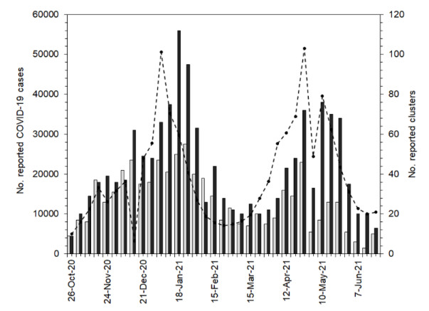
In Japan, a prioritized COVID-19 vaccination program using Pfizer/BioNTech messenger RNA (mRNA) vaccine among healthcare workers commenced on February 17, 2021. As vaccination coverage increases, clusters in healthcare and elderly care facilities including hospitals and nursing homes are expected to be reduced. The present study aimed to explicitly estimate the protective effect of vaccination in reducing cluster incidence in those facilities. A mathematical model was formulated using three pieces of information: (1) the incidence of clusters in facilities from October 26, 2020 to June 27, 2021; (2) the incidence of confirmed COVID-19 cases during the same period; and (3) vaccine doses among healthcare workers from February 17 to June 27, 2021, extracted from the national Vaccination System database. We found that the estimated proportion at risk in healthcare and elderly care facilities declined substantially as the vaccination coverage among healthcare workers increased; the greater risk reduction was observed in healthcare facilities, at 0.10 (95% confidence interval (CI): 0.04–0.16) times that in the pre-vaccination period, while that in elderly care facilities was 0.34 (95% CI: 0.24–0.43) times that in the earlier period. The averted numbers of clusters in healthcare facilities and elderly care facilities were estimated to be 247 (95% CI: 210–301) and 279 (95% CI: 218–354), respectively. Prioritized vaccination among healthcare workers had a marked impact on preventing the incidence of clusters in facilities.
Citation: Misaki Sasanami, Taishi Kayano, Hiroshi Nishiura. The number of COVID-19 clusters in healthcare and elderly care facilities averted by vaccination of healthcare workers in Japan, February–June 2021[J]. Mathematical Biosciences and Engineering, 2022, 19(3): 2762-2773. doi: 10.3934/mbe.2022126
In Japan, a prioritized COVID-19 vaccination program using Pfizer/BioNTech messenger RNA (mRNA) vaccine among healthcare workers commenced on February 17, 2021. As vaccination coverage increases, clusters in healthcare and elderly care facilities including hospitals and nursing homes are expected to be reduced. The present study aimed to explicitly estimate the protective effect of vaccination in reducing cluster incidence in those facilities. A mathematical model was formulated using three pieces of information: (1) the incidence of clusters in facilities from October 26, 2020 to June 27, 2021; (2) the incidence of confirmed COVID-19 cases during the same period; and (3) vaccine doses among healthcare workers from February 17 to June 27, 2021, extracted from the national Vaccination System database. We found that the estimated proportion at risk in healthcare and elderly care facilities declined substantially as the vaccination coverage among healthcare workers increased; the greater risk reduction was observed in healthcare facilities, at 0.10 (95% confidence interval (CI): 0.04–0.16) times that in the pre-vaccination period, while that in elderly care facilities was 0.34 (95% CI: 0.24–0.43) times that in the earlier period. The averted numbers of clusters in healthcare facilities and elderly care facilities were estimated to be 247 (95% CI: 210–301) and 279 (95% CI: 218–354), respectively. Prioritized vaccination among healthcare workers had a marked impact on preventing the incidence of clusters in facilities.

| [1] |
L. H. Nguyen, D. A. Drew, M. S. Graham, A. D. Joshi, C. G. Guo, W. Ma, et al., Risk of COVID-19 among front-line health-care workers and the general community: A prospective cohort study, Lancet Public Health, 5 (2020), e475–e483. doi: 10.1016/S2468-2667(20)30164-X. doi: 10.1016/S2468-2667(20)30164-X

|
| [2] |
R. E. Jordan, P. Adab, K. K. Cheng, Covid-19: Risk factors for severe disease and death, BMJ, 368 (2020), 1–2. doi: 10.1136/bmj.m1198. doi: 10.1136/bmj.m1198
|
| [3] |
T. M. Mcmichael, S. Clark, S. Pogosjans, M. Kay, J. Lewis, A. Baer, COVID-19 in a long-term care facility—King County, Washington, MMWR. Morb. Mortal. Wkly. Rep., 69 (2020), 339–342. doi: 10.15585/mmwr.mm6912e1. doi: 10.15585/mmwr.mm6912e1
|
| [4] |
S. N. Ladhani, J. Y. Chow, R. Janarthanan, J. Fok, E. Crawley-Boevey, A. Vusirikala, et al., Investigation of SARS-CoV-2 outbreaks in six care homes in London, April 2020, EClinicalMedicine, 26 (2020), 100533. doi: 10.1016/j.eclinm.2020.100533. doi: 10.1016/j.eclinm.2020.100533
|
| [5] | A. Comas-herrera, J. Zalakaín, E. Lemmon, C. Litwin, A. T. Hsu, A. E. Schmidt, et al., Mortality associated with COVID-19 in care homes: International evidence, Int. Long-Term Care Policy Netw., (2020), 1–30. Available from: https://ltccovid.org/wp-content/uploads/2020/10/Mortality-associated-with-COVID-among-people-living-in-care-homes-14-October-2020-4.pdf. |
| [6] |
V. J. Hall, S. Foulkes, A. Saei, N. Andrews, B. Oguti, A. Charlett, et al., COVID-19 vaccine coverage in health-care workers in England and effectiveness of BNT162b2 mRNA vaccine against infection (SIREN): A prospective, multicentre, cohort study, Lancet., 397 (2021), 1725–1735. doi: 10.1016/S0140-6736(21)00790-X. doi: 10.1016/S0140-6736(21)00790-X
|
| [7] |
M. G. Thompson, J. L. Burgess, A. L. Naleway, H. L. Tyner, S. K. Yoon, J. Meece, et al., Interim estimates of vaccine effectiveness of BNT162b2 and mRNA-1273 COVID-19 vaccines in preventing SARS-CoV-2 infection among health care personnel, first responders, and other essential and frontline workers—Eight U.S. locations, December 2020–March, MMWR. Morb. Mortal. Wkly. Rep., 70 (2021), 495–500. doi: 10.15585/mmwr.mm7013e3. doi: 10.15585/mmwr.mm7013e3
|
| [8] |
E. J. Haas, F. J. Angulo, J. M. McLaughlin, E. Anis, S. R. Singer, F. Khan, et al., Impact and effectiveness of mRNA BNT162b2 vaccine against SARS-CoV-2 infections and COVID-19 cases, hospitalisations, and deaths following a nationwide vaccination campaign in Israel: An observational study using national surveillance data, Lancet, 397 (2021), 1819–1829. doi: 10.1016/S0140-6736(21)00947-8. doi: 10.1016/S0140-6736(21)00947-8
|
| [9] |
F. P. Polack, S. J. Thomas, N. Kitchin, J. Absalon, A. Gurtman, S. Lockhart, et al., Safety and efficacy of the BNT162b2 mRNA Covid-19 vaccine, N. Engl. J. Med., 383 (2020), 2603–2615. doi: 10.1056/nejmoa2034577. doi: 10.1056/nejmoa2034577
|
| [10] |
N. Dagan, N. Barda, E. Kepten, O. Miron, S. Perchik, M. A. Katz, et al., BNT162b2 mRNA Covid-19 vaccine in a nationwide mass vaccination setting, N. Engl. J. Med., 384 (2021), 1412–1423. doi: 10.1056/nejmoa2101765. doi: 10.1056/nejmoa2101765
|
| [11] |
J.L. Bernal, N. Andrews, C. Gower, C. Robertson, J. Stowe, E. Tessier, et al., Effectiveness of the Pfizer-BioNTech and Oxford-AstraZeneca vaccines on covid-19 related symptoms, hospital admissions, and mortality in older adults in England: Test negative case-control study, BMJ, 373 (2021). doi: 10.1136/bmj.n1088. doi: 10.1136/bmj.n1088
|
| [12] |
A. Britton, K. M. J. Slifka, C. Edens, S. A. Nanduri, S. M. Bart, N. Shang, et al., Effectiveness of the Pfizer-BioNTech COVID-19 vaccine among residents of two skilled nursing facilities experiencing COVID-19 outbreaks—Connecticut, December 2020-February 2021, MMWR Recomm. Reports, 70 (2021), 396–401. doi: 10.15585/mmwr.mm7011e3. doi: 10.15585/mmwr.mm7011e3
|
| [13] |
R. J. Harris, J. A. Hall, A. Zaidi, N. J. Andrews, J. K. Dunbar, G. Dabrera, Effect of vaccination on household transmission of SARS-CoV-2 in England, N. Engl. J. Med., 385 (2021), 759–760. doi: 10.1056/nejmc2107717. doi: 10.1056/nejmc2107717
|
| [14] | J. Salo, M. Hägg, M. Kortelainen, T. Leino, T. Saxell, M. Siikanen, et al., The indirect effect of mRNA-based Covid-19 vaccination on unvaccinated household members, unpublished work. doi: 10.1101/2021.05.27.21257896. |
| [15] |
A. S. V. Shah, C. Gribben, J. Bishop, P. Hanlon, D. Caldwell, R. Wood, et al., Effect of vaccination on transmission of SARS-CoV-2, N. Engl. J. Med., 385 (2021), 1718–1720. doi: 10.1056/NEJMc2106757. doi: 10.1056/NEJMc2106757
|
| [16] |
O. Milman, I. Yelin, N. Aharony, R. Katz, E. Herzel, A. Ben-Tov, et al., Community-level evidence for SARS-CoV-2 vaccine protection of unvaccinated individuals, Nat. Med., 27 (2021), 1367–1369. doi: 10.1038/s41591-021-01407-5. doi: 10.1038/s41591-021-01407-5
|
| [17] | Public Health England, Direct and indirect impact of the vaccination programme on COVID-19 infections and mortality, 2021. Available from: https://assets.publishing.service.gov.uk/government/uploads/system/uploads/attachment_data/file/997495/Impact_of_COVID-19_vaccine_on_infection_and_mortality.pdf |
| [18] | Ministry of Health Labour and Welfare, Infection prevention and healthcare system development. Available from: https://www.mhlw.go.jp/stf/covid-19/kansenkakudaiboushi-iryouteikyou.html. |
| [19] |
Y. Furuse, E. Sando, N. Tsuchiya, R. Miyahara, I. Yasuda, Y.K. Ko, et al., Clusters of coronavirus disease in communities, Japan, January–April 2020, Emerg. Infect. Dis., 26 (2020), 13–16. doi: 10.3201/eid2609.202272. doi: 10.3201/eid2609.202272
|
| [20] | National Institute of Infectious Diseases, COVID-19 cluster prevention measures, 2020. Available from: https://www.niid.go.jp/niid/ja/typhi-m/iasr-reference/2523-related-articles/related-articles-485/9756-485r03.html. |
| [21] | Ministry of Health Labour and Welfare, Visualizing the data: information on COVID-19 infections. Available from: https://covid19.mhlw.go.jp/en/. |
| [22] | National Institute of Infectious Diseases, About new concerning variant of SARS-CoV-2 that may have different infectiousness, transmissibility, and antigenicity (9th report), 2021. Available from: https://www.niid.go.jp/niid/ja/2019-ncov/2484-idsc/10434-covid19-43.html. |
| [23] | Prime Minister's Office of Japan, About COVID-19 vaccine rollout schedule. Available from: https://www.kantei.go.jp/jp/headline/kansensho/vaccine_supply.html. |
| [24] | Ministry of Health Labour and Welfare, About vaccination of healthcare workers. Available from: https://www.mhlw.go.jp/stf/seisakunitsuite/bunya/vaccine_iryoujuujisha.html. |
| [25] | Ministry of Health Labour and Welfare, Effective distribution of vaccines for healthcare workers (amended), 2021. Available from: https://www.mhlw.go.jp/content/000786364.pdf. |
| [26] | Ministry of Health Labour and Welfare, About questions and answers (Q & A) regarding "Effective distribution of vaccines for healthcare workers (amended)", 2021. Available from: https://www.mhlw.go.jp/content/000793279.pdf. |
| [27] |
S. Bagchi, J. Mak, Q. Li, E. Sheriff, E. Mungai, A. Anttila, et al., Rates of COVID-19 among residents and staff members in nursing homes—United States, May 25–November 22, 2020, MMWR. Morb. Mortal. Wkly. Rep., 70 (2021), 52–55. doi: 10.15585/mmwr.mm7002e2. doi: 10.15585/mmwr.mm7002e2
|
| [28] | Ministry of Health Labour and Welfare, COVID-19 Vaccines. Available from: https://www.mhlw.go.jp/stf/covid-19/vaccine.html. |
| [29] |
A. Sheikh, J. McMenamin, B. Taylor, C. Robertson, SARS-CoV-2 Delta VOC in Scotland: demographics, risk of hospital admission, and vaccine effectiveness, Lancet, 397 (2021), 2461–2462. doi: 10.1016/S0140-6736(21)01358-1. doi: 10.1016/S0140-6736(21)01358-1
|
| [30] | Prime Minister's Office of Japan, About COVID-19 vaccination. Available from: https://www.kantei.go.jp/jp/headline/kansensho/vaccine.html. |


Figures(4)

Misaki Sasanami, Taishi Kayano, Hiroshi Nishiura. The number of COVID-19 clusters in healthcare and elderly care facilities averted by vaccination of healthcare workers in Japan, February–June 2021[J]. Mathematical Biosciences and Engineering, 2022, 19(3): 2762-2773. doi: 10.3934/mbe.2022126


 DownLoad: