Program-wide binary code diffing is widely used in the binary analysis field, such as vulnerability detection. Mature tools, including BinDiff and TurboDiff, make program-wide diffing using rigorous comparison basis that varies across versions, optimization levels and architectures, leading to a relatively inaccurate comparison result. In this paper, we propose a program-wide binary diffing method based on neural network model that can make diffing across versions, optimization levels and architectures. We analyze the target comparison files in four different granularities, and implement the diffing by both top down process and bottom up process according to the granularities. The top down process aims to narrow the comparison scope, selecting the candidate functions that are likely to be similar according to the call relationship. Neural network model is applied in the bottom up process to vectorize the semantic features of candidate functions into matrices, and calculate the similarity score to obtain the corresponding relationship between functions to be compared. The bottom up process improves the comparison accuracy, while the top down process guarantees efficiency. We have implemented a prototype PBDiff and verified its better performance compared with state-of-the-art BinDiff, Asm2vec and TurboDiff. The effectiveness of PBDiff is further illustrated through the case study of diffing and vulnerability detection in real-world firmware files.
Citation: Lu Yu, Yuliang Lu, Yi Shen, Jun Zhao, Jiazhen Zhao. PBDiff: Neural network based program-wide diffing method for binaries[J]. Mathematical Biosciences and Engineering, 2022, 19(3): 2774-2799. doi: 10.3934/mbe.2022127
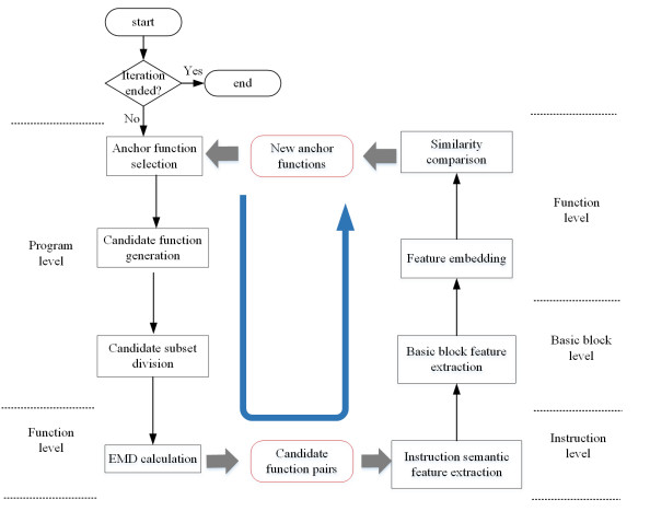
Program-wide binary code diffing is widely used in the binary analysis field, such as vulnerability detection. Mature tools, including BinDiff and TurboDiff, make program-wide diffing using rigorous comparison basis that varies across versions, optimization levels and architectures, leading to a relatively inaccurate comparison result. In this paper, we propose a program-wide binary diffing method based on neural network model that can make diffing across versions, optimization levels and architectures. We analyze the target comparison files in four different granularities, and implement the diffing by both top down process and bottom up process according to the granularities. The top down process aims to narrow the comparison scope, selecting the candidate functions that are likely to be similar according to the call relationship. Neural network model is applied in the bottom up process to vectorize the semantic features of candidate functions into matrices, and calculate the similarity score to obtain the corresponding relationship between functions to be compared. The bottom up process improves the comparison accuracy, while the top down process guarantees efficiency. We have implemented a prototype PBDiff and verified its better performance compared with state-of-the-art BinDiff, Asm2vec and TurboDiff. The effectiveness of PBDiff is further illustrated through the case study of diffing and vulnerability detection in real-world firmware files.

| [1] | Synopsys 2020 open source security and risk analysis report, 2020. Avaiable from: https://www.synopsys.com/software-integrity/resources/analyst-reports/2020-open-source-security-risk-analysis.html?cmp=pr-sig. |
| [2] | Eliminating vulnerabilities in third-party code with binary analysis, 2020. Avaiable from: https://codesonar.grammatech.com/eliminating-vulnerabilities-in-third-party-code-with-binary-analysis. |
| [3] | Breaking down mirai: An iot ddos botnet, 2020. Avaiable from: https://www.imperva.com/blog/malware-analysis-mirai-ddos-botnet/. |
| [4] | Diaphora, 2020. Avaiable from: https://github.com/joxeankoret/diaphora. |
| [5] | Zynamics bindiff, 2020. Avaiable from: https://www.zynamics.com/bindiff.html. |
| [6] | Turbodiff, 2020, Avaiable from https://www.coresecurity.com/core-labs/open-source-tools/turbodiff-cs. |
| [7] | Q. Feng, R. Zhou, C. Xu, Y. Cheng, B. Testa, H. Yin, Scalable graph-based bug search for firmware images, in Proceedings of the 2016 ACM SIGSAC Conference on Computer and Communications Security, ACM, (2016), 480–491. https://doi.org/10.1145/2976749.2978370 |
| [8] | X. Xu, C. Liu, Q. Feng, H. Yin, L. Song, D. Song, Neural network-based graph embedding for cross-platform binary code similarity detection, in Proceedings of the 2017 ACM SIGSAC Conference on Computer and Communications Security, ACM, (2017), 363–376. https://doi.org/10.1145/3133956.3134018 |
| [9] | J. Gao, X. Yang, Y. Fu, Y. Jiang, J. Sun, Vulseeker: a semantic learning based vulnerability seeker for cross-platform binary, in Proceedings of the 33rd ACM/IEEE International Conference on Automated Software Engineering, ACM, (2018), 896–899. https://doi.org/10.1145/3238147.3240480 |
| [10] | K. Redmond, L. Luo, Q. Zeng, A cross-architecture instruction embedding model for natural language, preprint, arXiv: 1812.09652. |
| [11] | Z. Yu, R. Cao, Q. Tang, S. Nie, J. Huang, S. Wu, Order matters: semantic-aware neural networks for binary code similarity detection, in Proceedings of the AAAI Conference on Artificial Intelligence, 34 (2020), 1145–1152. https://doi.org/10.1609/aaai.v34i01.5466 |
| [12] | Y. Bai, H. Ding, K. Gu, Y. Sun, W. Wang, Learning-based efficient graph similarity computation via multi-scale convolutional set matching, in Proceedings of the AAAI Conference on Artificial Intelligence, 34 (2020), 3219–3226. https://doi.org/10.1609/aaai.v34i04.5720 |
| [13] | Y. Duan, X. Li, J. Wang, H. Yin, Deepbindiff: Learning program-wide code representations for binary diffing, in Network and Distributed System Security Symposium, 2020. |
| [14] | S. H. Ding, B. C. Fung, P. Charland, Asm2vec: Boosting static representation robustness for binary clone search against code obfuscation and compiler optimization, in 2019 IEEE Symposium on Security and Privacy (SP), IEEE, (2019), 472–489. https://doi.org/10.1109/SP.2019.00003 |
| [15] | Z. Yu, W. Zheng, J. Wang, Q. Tang, S. Nie, S. Wu, Codecmr: Cross-modal retrieval for function-level binary source code matching, Adv. Neural Inf. Process. Syst., 33 (2020). |
| [16] | Y. Rubner, C. Tomasi, L. J. Guibas, A metric for distributions with applications to image databases, in Sixth International Conference on Computer Vision (IEEE Cat. No. 98CH36271), IEEE, (1998), 59–66. https://doi.org/10.1109/ICCV.1998.710701 |
| [17] |
D. Callahan, A. Carle, M. W. Hall, K. Kennedy, Constructing the procedure call multigraph, IEEE Trans. Software Eng., 16 (1990), 483–487. https://doi.org/10.1109/32.54302 doi: 10.1109/32.54302

|
| [18] | U. P. Khedker, A. Sanyal, B. Karkare, Data flow analysis: theory and practice, CRC Press, (2017). https://doi.org/10.1201/9780849332517 |
| [19] | L. Yu, Y. Shen, Z. Pan, Structure analysis of function call network based on percolation, in 2018 Eighth International Conference on Instrumentation and Measurement, Computer, Communication and Control (IMCCC), IEEE, (2018), 350–354. https://doi.org/10.1109/IMCCC.2018.00080 |
| [20] | R. Kiros, Y. Zhu, R. R. Salakhutdinov, R. Zemel, R. Urtasun, A. Torralba, et al., Skip-thought vectors, in Adv. Neural Inf. Process. Syst., (2015), 3294–3302. |
| [21] | T. N. Kipf, M. Welling, Variational graph auto-encoders, preprint, arXiv: 1611.07308. |
| [22] |
J. Bromley, J. W. Bentz, L. Bottou, I. Guyon, Y. LeCun, C. Moore, et al., Signature verification using a siamese time delay neural network, Intern. J. Pattern Recognit. Artif. Intell., 7 (1993), 669–688. https://doi.org/10.1142/S0218001493000339 doi: 10.1142/S0218001493000339
|
| [23] | H. Flake, Structural comparison of executable objects, in Detection of intrusions and malware and vulnerability assessment, DIMVA, (2004), 161–173. |
| [24] | D. Gao, M. K. Reiter, D. Song, Binhunt: Automatically finding semantic differences in binary programs, in International Conference on Information and Communications Security, Springer, (2008), 238–255. https://doi.org/10.1007/978-3-540-88625-9_16 |
| [25] | J. Ming, M. Pan, D. Gao, ibinhunt: Binary hunting with inter-procedural control flow, in International Conference on Information Security and Cryptology, Springer, (2012), 92–109. https://doi.org/10.1007/978-3-642-37682-5-8 |
| [26] |
Y. David, E. Yahav, Tracelet-based code search in executables, Acm Sigplan Not., 49 (2014), 349–360. https://doi.org/10.1145/2666356.2594343 doi: 10.1145/2666356.2594343
|
| [27] | L. Nouh, A. Rahimian, D. Mouheb, M. Debbabi, A. Hanna, Binsign: fingerprinting binary functions to support automated analysis of code executables, in IFIP International Conference on ICT Systems Security and Privacy Protection, Springer, (2017), 341–355. https://doi.org/10.1007/978-3-319-58469-0-23 |
| [28] | J. Pewny, B. Garmany, R. Gawlik, C. Rossow, T. Holz, Cross-architecture bug search in binary executables, in 2015 IEEE Symposium on Security and Privacy, IEEE, (2015), 709–724. https://doi.org/10.1109/SP.2015.49 |
| [29] | A. J. P. Tixier, G. Nikolentzos, P. Meladianos, M. Vazirgiannis, Graph classification with 2d convolutional neural networks, in International Conference on Artificial Neural Networks, Springer, (2019), 578–593. https://doi.org/10.1007/978-3-030-30493-5-54 |
| [30] | L. Wang, B. Zong, Q. Ma, W. Cheng, J. Ni, W. Yu, et al., Inductive and unsupervised representation learning on graph structured objects, in International Conference On Learning Representations, 2020. |
| [31] | S. Liu, M. F. Demirel, Y. Liang, N-gram graph: Simple unsupervised representation for graphs, with applications to molecules, preprint, arXiv: 1806.09206. |
| [32] | Y. Li, C. Gu, T. Dullien, O. Vinyals, P. Kohli, Graph matching networks for learning the similarity of graph structured objects, in International Conference on Machine Learning, PMLR, (2019), 3835–3845. |
| [33] | R. Wang, J. Yan, X. Yang, Learning combinatorial embedding networks for deep graph matching, in Proceedings of the IEEE/CVF International Conference on Computer Vision, (2019), 3056–3065. |
| [34] | B. Jiang, P. Sun, J. Tang, B. Luo, Glmnet: Graph learning-matching networks for feature matching, preprint, arXiv: 1911.07681. |
| [35] | H. Zhang, Z. Qian, Precise and accurate patch presence test for binaries, in 27th USENIX Security Symposium, (2018), 887–902. |
| [36] | S. C. Wang, C. L. Liu, Y. Li, W. Y. Xu, Semdiff: Finding semtic differences in binary programs based on angr, in ITM Web of Conferences, 12 (2017), 03029. https://doi.org/10.1051/itmconf/20171203029 |
| [37] | C. Yang, Z. Liu, D. Zhao, M. Sun, E. Chang, Network representation learning with rich text information, in Twenty-fourth international joint conference on artificial intelligence, (2015), 2111–2117. |
| [38] | F. Zuo, X. Li, P. Young, L. Luo, Q. Zeng, Z. Zhang, Neural machine translation inspired binary code similarity comparison beyond function pairs, preprint, arXiv: 1808.04706. |
| [39] |
S. Alrabaee, P. Shirani, L. Wang, M. Debbabi, Sigma: A semantic integrated graph matching approach for identifying reused functions in binary code, Digital Invest., 12 (2015), S61–S71. https://doi.org/10.1016/j.diin.2015.01.011 doi: 10.1016/j.diin.2015.01.011
|
| [40] |
R. Li, C. Zhang, C. Feng, X. Zhang, C. Tang, Locating vulnerability in binaries using deep neural networks, Ieee Access, 7 (2019), 134660–134676. https://doi.org/10.1109/ACCESS.2019.2942043 doi: 10.1109/ACCESS.2019.2942043
|
| [41] |
Y. Hu, H. Wang, Y. Zhang, B. Li and D. Gu, A semantics-based hybrid approach on binary code similarity comparison, IEEE Trans. Software Eng., 47(2021), 1241-1258. https://doi.org/10.1109/TSE.2019.2918326 doi: 10.1109/TSE.2019.2918326
|
| [42] | S. H. Ding, B. C. Fung, P. Charland, Kam1n0: Mapreduce-based assembly clone search for reverse engineering, in Proceedings of the 22nd ACM SIGKDD International Conference on Knowledge Discovery and Data Mining, (2016), 461–470. https://doi.org/10.1145/2939672.2939719 |
| [43] | Y. Li, J. Jang and X. Ou, Topology-aware hashing for effective control flow graph similarity analysis, in International Conference on Security and Privacy in Communication Systems, Springer, (2019), 278–298. https://doi.org/10.1007/978-3-030-37228-6-14 |


Figures(8) / Tables(4)

Lu Yu, Yuliang Lu, Yi Shen, Jun Zhao, Jiazhen Zhao. PBDiff: Neural network based program-wide diffing method for binaries[J]. Mathematical Biosciences and Engineering, 2022, 19(3): 2774-2799. doi: 10.3934/mbe.2022127


 DownLoad: