Distortional buckling behavior and design method of cold-formed steel lipped channel with rectangular holes under axial compression

Yanli Guo; Xingyou Yao; Yanli Guo; Xingyou Yao

doi:10.3934/mbe.2021312

Mathematical Biosciences and Engineering

2021, Volume 18, Issue 5: 6239-6261. doi: 10.3934/mbe.2021312

Previous Article Next Article

Research article

Distortional buckling behavior and design method of cold-formed steel lipped channel with rectangular holes under axial compression

Yanli Guo ^{1
,
,},
Xingyou Yao ²

1.
School of Civil Engineering and Architecture, Nanchang University, Nanchang, Jiangxi 330000, China
2.
Jiangxi Province Key Laboratory of Hydraulic and Civil Engineering Infrastructure Security, Nanchang Institute of Technology, Nanchang, Jiangxi 330000, China

Academic Editor: Xiaodong Huang

Received: 21 June 2021 Accepted: 12 July 2021 Published: 19 July 2021

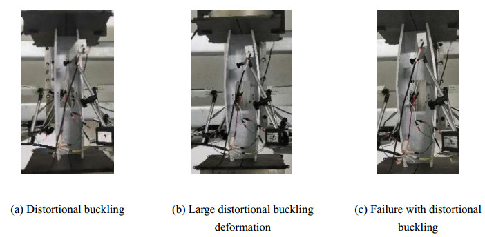
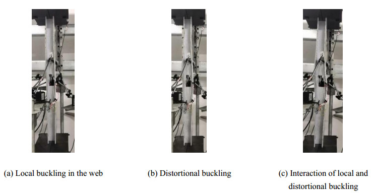
The use of cold-formed steel (CFS) channel sections with rectangular holes in the web is becoming gradually popular in building structures. However, such holes can result in sections becoming more susceptible to be distortional buckling and display lower load-carrying capacities. This paper presents a total of 44 axially-compressed tests of CFS lipped channel columns with and without rectangular web holes including different hole sizes and cross-sections. The test results show that the specimens were controlled by distortional buckling or interaction of local buckling and distortional buckling. The load-carrying capacities of specimens with rectangular holes were lower than that of specimens without hole. The load-carrying capacities of specimens were gradually decreased with the increasing of dimensions of holes. Then a nonlinear elasto-plastic finite element model (FEM) was developed and the analysis results showed good agreement with the test results. The validated FE model was used to conduct a parametric study involving 16 FEM to investigate the effects of the section, the dimension of the hole, and the number of holes on the ultimate strength of such channels. Furthermore, the formulas to predict the distortional buckling coefficient were developed for the section with holes by using the verified FEM. Finally, the tests and parametric study results were compared against the distortional buckling design strengths calculated in accordance with the developed method. The comparison results show that the proposed design method closely predict the load carrying capacity of CFS channel sections with rectangular web holes.

Keywords:

Citation: Yanli Guo, Xingyou Yao. Distortional buckling behavior and design method of cold-formed steel lipped channel with rectangular holes under axial compression[J]. Mathematical Biosciences and Engineering, 2021, 18(5): 6239-6261. doi: 10.3934/mbe.2021312

Related Papers:

[1]	Yantao Song, Wenjie Zhang, Yue Zhang . A novel lightweight deep learning approach for simultaneous optic cup and optic disc segmentation in glaucoma detection. Mathematical Biosciences and Engineering, 2024, 21(4): 5092-5117. doi: 10.3934/mbe.2024225
[2]	Rafsanjany Kushol, Md. Hasanul Kabir, M. Abdullah-Al-Wadud, Md Saiful Islam . Retinal blood vessel segmentation from fundus image using an efficient multiscale directional representation technique Bendlets. Mathematical Biosciences and Engineering, 2020, 17(6): 7751-7771. doi: 10.3934/mbe.2020394
[3]	Yue Li, Hongmei Jin, Zhanli Li . A weakly supervised learning-based segmentation network for dental diseases. Mathematical Biosciences and Engineering, 2023, 20(2): 2039-2060. doi: 10.3934/mbe.2023094
[4]	Jianguo Xu, Cheng Wan, Weihua Yang, Bo Zheng, Zhipeng Yan, Jianxin Shen . A novel multi-modal fundus image fusion method for guiding the laser surgery of central serous chorioretinopathy. Mathematical Biosciences and Engineering, 2021, 18(4): 4797-4816. doi: 10.3934/mbe.2021244
[5]	Dehua Feng, Xi Chen, Xiaoyu Wang, Xuanqin Mou, Ling Bai, Shu Zhang, Zhiguo Zhou . Predicting effectiveness of anti-VEGF injection through self-supervised learning in OCT images. Mathematical Biosciences and Engineering, 2023, 20(2): 2439-2458. doi: 10.3934/mbe.2023114
[6]	Ran Zhou, Yanghan Ou, Xiaoyue Fang, M. Reza Azarpazhooh, Haitao Gan, Zhiwei Ye, J. David Spence, Xiangyang Xu, Aaron Fenster . Ultrasound carotid plaque segmentation via image reconstruction-based self-supervised learning with limited training labels. Mathematical Biosciences and Engineering, 2023, 20(2): 1617-1636. doi: 10.3934/mbe.2023074
[7]	Duolin Sun, Jianqing Wang, Zhaoyu Zuo, Yixiong Jia, Yimou Wang . STS-TransUNet: Semi-supervised Tooth Segmentation Transformer U-Net for dental panoramic image. Mathematical Biosciences and Engineering, 2024, 21(2): 2366-2384. doi: 10.3934/mbe.2024104
[8]	Zhenwu Xiang, Qi Mao, Jintao Wang, Yi Tian, Yan Zhang, Wenfeng Wang . Dmbg-Net: Dilated multiresidual boundary guidance network for COVID-19 infection segmentation. Mathematical Biosciences and Engineering, 2023, 20(11): 20135-20154. doi: 10.3934/mbe.2023892
[9]	Wenli Cheng, Jiajia Jiao . An adversarially consensus model of augmented unlabeled data for cardiac image segmentation (CAU⁺). Mathematical Biosciences and Engineering, 2023, 20(8): 13521-13541. doi: 10.3934/mbe.2023603
[10]	Jingyao Liu, Qinghe Feng, Yu Miao, Wei He, Weili Shi, Zhengang Jiang . COVID-19 disease identification network based on weakly supervised feature selection. Mathematical Biosciences and Engineering, 2023, 20(5): 9327-9348. doi: 10.3934/mbe.2023409

Abstract

1. Introduction

To exemplify the phenomena of compounds scientifically, researchers utilize the contraption of the diagrammatic hypothesis, it is a well-known branch of geometrical science named graph theory. This division of numerical science provides its services in different fields of sciences. The particular example in networking ^[1], from electronics ^[2], and for the polymer industry, we refer to see ^[3]. Particularly in chemical graph theory, this division has extra ordinary assistance to study giant and microscope-able chemical compounds. For such a study, researchers made some transformation rules to transfer a chemical compound to a discrete pattern of shapes (graph). Like, an atom represents as a vertex and the covalent bonding between atoms symbolized as edges. Such transformation is known as molecular graph theory. A major importance of this alteration is that the hydrogen atoms are omitted. Some chemical structures and compounds conversion are presented in ^[4,5,6].

In cheminformatics, the topological index gains attraction due to its implementations. Various topological indices help to estimate a bio-activity and physicochemical characteristics of a chemical compound. Some interesting and useful topological indices for various chemical compounds are studied in ^[3,7,8]. A topological index modeled a molecular graph or a chemical compound into a numerical value. Since 1947, topological index implemented in chemistry ^[9], biology ^[10], and information science ^[11,12]. Sombor index and degree-related properties of simplicial networks ^[13], Nordhaus–Gaddum-type results for the Steiner Gutman index of graphs ^[14], Lower bounds for Gaussian Estrada index of graphs ^[15], On the sum and spread of reciprocal distance Laplacian eigenvalues of graphs in terms of Harary index ^[16], the expected values for the Gutman index, Schultz index, and some Sombor indices of a random cyclooctane chain ^[17,18,19], bounds on the partition dimension of convex polytopes ^[20,21], computing and analyzing the normalized Laplacian spectrum and spanning tree of the strong prism of the dicyclobutadieno derivative of linear phenylenes ^[22], on the generalized adjacency, Laplacian and signless Laplacian spectra of the weighted edge corona networks ^[23,24], Zagreb indices and multiplicative Zagreb indices of Eulerian graphs ^[25], Minimizing Kirchhoff index among graphs with a given vertex bipartiteness, ^[26], asymptotic Laplacian energy like invariant of lattices ^[27]. Few interesting studies regarding the chemical graph theory can be found in ^{[28,29,30,31,32]}.

Recently, the researchers of ^[33] introduced a topological descriptor and called the face index. Moreover, the idea of computing structure-boiling point and energy of a structure, motivated them to introduced this parameter without heavy computation. They computed these parameters for different models compare the results with previous literature and found approximate solutions with comparatively less computations. This is all the blessings of face index of a graph. The major concepts of this research work are elaborated in the given below definitions.

Definition 1.1. ^[33] Let a graph $G = \left(V(G), E(G), F(G)\right)$ having face, edge and vertex sets notation with $F(G), E(G), V(G),$ respectively. It is mandatory that the graph is connected, simple and planar. If $e$ from the edge set $E(G),$ is one of those edges which surrounds a face, then the face $f$ from the face set $F(G),$ is incident to the edge $e.$ Likewise, if a vertex $\alpha$ from the vertex set $V(G)$ is at the end of those incident edges, then a face $f$ is incident to that vertex. This face-vertex incident relation is symbolized here by the notation $\alpha\sim f.$ The face degree of $f$ in $G$ is described as $d(f) = \sum_{\alpha\sim f}{d\left(\alpha\right)},$ which are elaborated in the Figure 1.

Figure 1. An example of face degree.

DownLoad: Full-Size Img PowerPoint

Definition 1.2. ^[33] The face index $FI\left(G\right),$ for a graph $G,$ is formulated as

$\begin{equation*} FI\left(G\right) = \sum\limits_{f\in F\left(G\right)}{d(f)} = \sum\limits_{\alpha\sim f, f\in F(G)}{d\left(\alpha\right)}. \end{equation*}$

In the , we can see that there are two faces with degree $4,$ exactly two with five count and four with count of 6. Moreover, there is an external face with count of face degree $28,$ which is the count of vertices.

As the information given above that the face index is quite new and introduced in the year 2020, so there is not so much literature is available. A few recent studies on this topic are summarized here. A chemical compound of silicon carbides is elaborated with such novel definition in ^[34]. Some carbon nanotubes are discussed in ^[35]. Except for the face index, there are distance and degree-based graphical descriptors available in the literature. For example, distance-based descriptors of phenylene nanotube are studied in ^[36], and in ^[37] titania nanotubes are discussed with the same concept. Star networks are studied in ^[38], with the concept of degree-based descriptors. Bounds on the descriptors of some generalized graphs are discussed in ^[39]. General Sierpinski graph is discussed in ^[40], in terms of different topological descriptor aspects. The study of hyaluronic acid-doxorubicin ar found in ^[41], with the same concept of the index. The curvilinear regression model of the topological index for the COVID-19 treatment is discussed in ^[42]. For further reading and interesting advancements of topological indices, polynomials of zero-divisor structures are found in ^[43], zero divisor graph of commutative rings ^[44], swapped networks modeled by optical transpose interconnection system ^[45], metal trihalides network ^[46], some novel drugs used in the cancer treatment ^[47], para-line graph of Remdesivir used in the prevention of corona virus ^[48], tightest nonadjacently configured stable pentagonal structure of carbon nanocones ^[49]. In order to address a novel preventive category (P) in the HIV system known as the HIPV mathematical model, the goal of this study is to offer a design of a Morlet wavelet neural network (MWNN) ^[50].

In the next section, we discussed the newly developed face index or face-based index for different chemical compounds. Silicate network, triangular honeycomb network, carbon sheet, polyhedron generalized sheet, and generalized chain of silicate network are studied with the concept of the face-based index. Given that the face index is more versatile than vertex degree-based topological descriptors, this study will aid in understanding the structural characteristics of chemical networks. Only the difficulty authors will face to compute the face degree of a generalized network or structure, because it is more generalized version and taking degree based partition of edges into this umbrella of face index.

2. Results on the face index of chemical networks

Silicates are formed when metal carbonates or metal oxides react with sand. The $SiO_4,$ which has a tetrahedron structure, is the fundamental chemical unit of silicates. The central vertex of the $SiO_4$ tetrahedron is occupied by silicon ions, while the end vertices are occupied by oxygen ions ^[51,52,53]. A silicate sheet is made up of rings of tetrahedrons that are joined together in a two-dimensional plane by oxygen ions from one ring to the other to form a sheet-like structure. The silicate network $SL_{n}$ symbol, where ${n}$ represents the total number of hexagons occurring between the borderline and center of the silicate network $SL_{n}.$ The silicate network of dimension one is depicted in . It contain total $3{n}\left(5{n}+1\right)$ vertices are $36{n}^2$ edges. Moreover, the result required is detailed are available in Table 1.

Figure 2. A silicate network

$SL_{1}$ .

DownLoad: Full-Size Img PowerPoint

Table 1. The number of

$f_{12},$

$f_{15}$ and

$f_{36}$ in each dimension.

Dimension	${\bf{\|}}{\boldsymbol{f}}_{{\bf{12}}}{\bf{\|}}$	${\bf{\|}}{\boldsymbol{f}}_{{\bf{15}}}{\bf{\|}}$	${\bf{\|}}{\boldsymbol{f}}_{{\bf{36}}}{\bf{\|}}$
$1$	$24$	$48$	$7$
$2$	$32$	$94$	$14$
$3$	$40$	$152$	$23$
$4$	$48$	$222$	$34$
$5$	$56$	$304$	$47$
$6$	$64$	$398$	$62$
$7$	$72$	$504$	$79$
$8$	$80$	$622$	$98$
.	.	.	.
.	.	.	.
.	.	.	.
${n}$	$8{n}+16$	$6{n}^{2}+28{n}+14$	${n}^{2}+4{n}+2$

| Show Table

DownLoad: CSV

Theorem 2.1. Let $SL_{n}$ be the silicate network of dimension $n\geq1.$ Then the face index of $SL_{n}$ is

$\begin{equation*} FI\left(SL_{n}\right) = 126{n}^{2}+720{n}+558. \end{equation*}$

Proof. Consider $SL_{n}$ the graph of silicate network with dimension ${n}.$ Suppose $f_{i}$ denotes the faces of graph $SL_{n}$ having degree $i.$ that is, $d(f_{i}) = \sum_{\alpha\sim f_{i}}{d\left(\alpha\right)} = i$ and $|f_{i}|$ denotes the number of faces with degree $i.$ The graph $SL_{n}$ contains three types of internal faces $f_{12},$ $f_{15},$ $f_{36},$ and single external face which is usually denoted by $f^{\infty}.$

If $SL_{n}$ has one dimension then sum of degree of vertices incident to the external face is $144$ and when $SL_{n}$ has two dimension then sum of degree of incident vertices to the external face is $204$ whenever $SL_{n}$ has three dimension then sum of degree of incident vertices to the external face is $264.$ Similarly, $SL_{n}$ has $n-$ dimension then sum of degree of incident vertices to the external face is $60n+84.$

The number of internal faces with degree in each dimension is mentioned in Table 1.

By using the definition of face index $FI$ we have

$\begin{align*} FI\left(SL_{n}\right) = &\sum\limits_{\alpha\sim f\in F\left(SL_{n}\right)}{d\left(\alpha\right)}\\ = &\sum\limits_{\alpha\sim f_{12}\in F\left(SL_{n}\right)}{d\left(\alpha\right)}+ \sum\limits_{\alpha\sim f_{15}\in F\left(SL_{n}\right)}{d\left(\alpha\right)}+ \sum\limits_{\alpha\sim f_{36}\in F\left(SL_{n}\right)}{d\left(\alpha\right)}+ \sum\limits_{\alpha\sim f^{\infty}\in F\left(SL_{n}\right)}{d\left(\alpha\right)}\\ = &|f_{12}|(12)+|f_{15}|(15)+|f_{36}|(36)+(60n+84)\\ = &(8n+16)(12)+(6n^{2}+28n+14)(15)+(n^{2}+4n+2)(36)+60n+84\\ = &126n^{2}+72n+558. \end{align*}$

Hence, this is our required result.

A chain silicate network of dimension $(m, n)$ is symbolized as $CSL\left(m, n\right)$ which is made by arranging $(m, n)$ tetrahedron molecules linearly. A chain silicate network of dimension $(m, n)$ with $m, n\geq1$ where $m$ denotes the number of rows and each row has $n$ number of tetrahedrons. The following theorem formulates the face index $FI$ for chain silicate network.

Theorem 2.2. Let $CSL\left(m, n\right)$ be the chain of silicate network of dimension $m, n\geq1.$ Then the face index $FI$ of the graph $CSL\left(m, n\right)$ is

$\begin{equation*} FI\left(CSL\left(m, n\right)\right) = \begin{cases} 48n-12 & \text{if } m = 1, \ {n}\geq1; \\ 96m-12 & \text{if } n = 1, \ m\geq2; \\ 168m-60 & \text{if } n = 2, m\geq2; \\ 45m-9n+36mn-42 & \text{if } \text{both}\ m, n\ \text{are even} \\ 45m-9n+36mn-21 & \text{otherwise}. \end{cases} \end{equation*}$

Proof. Let $CSL\left(m, n\right)$ be the graph of chain silicate network of dimension $(m, n)$ with $m, n\geq1$ where $m$ represents the number of rows and $n$ is the number of tetrahedrons in each row. A graph $CSL\left(m, n\right)$ for $m = 1$ contains three type of internal faces $f_{9}, \ f_{12}$ and $f_{15}$ with one external face $f^{\infty}.$ While for $m\geq2,$ it has four type of internal faces $f_{9}, \ f_{12}, \ f_{15}$ and $f_{36}$ with one external face $f^{\infty}.$ We want to evaluate the algorithm of face index $FI$ for chain silicate network. We will discuss it in two different cases.

Case 1: When $CSL\left(m, n\right)$ has one row $(m = 1)$ with $n$ number of tetrahedrons as shown in the Figure 3.

Figure 3. Chain silicate network

$CSL\left(m, n\right)$ with particular value of

$m = 1$ .

DownLoad: Full-Size Img PowerPoint

The graph has three type of internal faces $f_{9}, \ f_{12}$ and $f_{15}$ with one external face $f^{\infty}.$ The sum of degree of incident vertices to the external face is $9n$ and number of faces are $|f_{9}| = 2, \ |f_{12}| = 2n$ and $|f_{15}| = n-2.$ Now the face index $FI$ of the graph $CSL\left(m, n\right)$ is given by

$\begin{align*} FI\left(CSL\left(m, n\right)\right) = &\sum\limits_{\alpha\sim f\in F\left(CSL\left(m, n\right)\right)}{d\left(\alpha\right)}\\ = &\sum\limits_{\alpha\sim f_{9}\in F\left(CSL\left(m, n\right)\right)}{d\left(\alpha\right)}+\sum\limits_{\alpha\sim f_{12}\in F\left(CSL\left(m, n\right)\right)}{d\left(\alpha\right)}+\sum\limits_{\alpha\sim f_{15}\in F\left(CSL\left(m, n\right)\right)}{d\left(\alpha\right)}\\&+\sum\limits_{\alpha\sim f^{\infty}\in F\left(CSL\left(m, n\right)\right)}{d\left(\alpha\right)}\\ = &|f_{9}|(9)+|f_{12}|(12)+|f_{15}|(15)+(9n)\\ = &(2)(9)+(2n)(12)+(n-2)(15)+9n\\ = &48n-12. \end{align*}$

Case 2: When $CSL\left(m, n\right)$ has more than one rows $(m\neq1)$ with $n$ number of tetrahedrons in each row as shown in the Figure 4.

Figure 4. Chain silicate network

$CSL\left(m, n\right)$ .

DownLoad: Full-Size Img PowerPoint

The graph has four type of internal faces $f_{9}, \ f_{12}, \ f_{15}$ and $f_{36}$ with one external face $f^{\infty}.$ The sum of degree of incident vertices to the external face is

$\begin{equation*} \sum\limits_{\alpha\sim f^{\infty}\in F\left(CSL\left(m, n\right)\right)}{d\left(\alpha\right)} = \begin{cases} 18m & \mbox{if } n = 1, \ m\geq1; \\ 27m & \mbox{if } n = 2, \ m\geq1; \\ 30m+15n-30 & \mbox{if } \text{both}\ m, n\ \text{are even} \\ 30m+15n-33 & {\text{otherwise}}. \end{cases} \end{equation*}$

The number of faces are $|f_{9}|, \ |f_{12}|, \ f_{15}$ and $|f_{36}|$ are given by

$\begin{align*} |f_{9}| = & \begin{cases} 2 & \mbox{if }\ m\ \text{is odd} \\ 3+(-1)^{n} & \mbox{if }\ m\ \text{is even}. \end{cases}\\ |f_{12}| = & \begin{cases} 2(2m+n-1) & \mbox{if}\ m\ \text{is odd} \\ 4(\lfloor\frac{n+1}{2}\rfloor+2m-1)& \mbox{if}\ m\ \text{is even} \end{cases}\\ |f_{15}| = &(3m-2)n-m\\ |f_{36}| = & \begin{cases} (\frac{m-1}{2})(n-1) & \mbox{if}\ m\ \text{is odd} \\ (\frac{2n+(-1)^{n}-1}{4})(\frac{m-2}{2})n & \mbox{if}\ m\ \text{is even}. \end{cases} \end{align*}$

Now the face index $FI$ of the graph $CSL\left(m, n\right)$ is given by

$\begin{align*} FI\left(CSL\left(m, n\right)\right) = &\sum\limits_{\alpha\sim f\in F\left(CSL\left(m, n\right)\right)}{d\left(\alpha\right)}\\ = &\sum\limits_{\alpha\sim f_{9}\in F\left(CSL\left(m, n\right)\right)}{d\left(\alpha\right)}+\sum\limits_{\alpha\sim f_{12}\in F\left(CSL\left(m, n\right)\right)}{d\left(\alpha\right)}+\sum\limits_{\alpha\sim f_{15}\in F\left(CSL\left(m, n\right)\right)}{d\left(\alpha\right)}\\&+\sum\limits_{\alpha\sim f_{36}\in F\left(CSL\left(m, n\right)\right)}{d\left(\alpha\right)}+\sum\limits_{\alpha\sim f^{\infty}\in F\left(CSL\left(m, n\right)\right)}{d\left(\alpha\right)}\\ = &|f_{9}|(9)+|f_{12}|(12)+|f_{15}|(15)+|f_{36}|(36)+\sum\limits_{\alpha\sim f^{\infty}\in F\left(CSL\left(m, n\right)\right)}{d\left(\alpha\right)}.\\ \end{align*}$

After some mathematical simplifications, we can get

$\begin{equation*} FI\left(CSL\left(m, n\right)\right) = \begin{cases} 48n-12 & \mbox{if } m = 1 \\ 96m-12 & \mbox{if } n = 1, \forall\;m \\ 168m-60 & \mbox{if } n = 2, \forall\;m \\ 45m-9n+36mn-42 & \mbox{if } \text{both}\ m, n\ \text{are even} \\ 45m-9n+36mn-21 & {\text{otherwise}}. \end{cases} \end{equation*}$

There are three regular plane tessellations known to exist, each constituted from the same type of regular polygon: triangular, square, and hexagonal. The triangular tessellation is used to define the hexagonal network, which is extensively studied in ^[54]. A dimensioned hexagonal network $TH_{k}$ has $3{k}^2-3{k}+1$ vertices and $9{k}^2-15{k}+6$ edges, where ${k}$ is the number of vertices on one side of the hexagon. It has $2{k}-2$ diameter. There are six vertices of degree three that are referred to as corner vertices. Moreover, the result required detailed are available in the Table 2.

Figure 5. Triangular honeycomb network with dimension

${k}=3$ .

DownLoad: Full-Size Img PowerPoint

Table 2. The number of

$f_{12},$

$f_{14},$

$f_{17}$ and

$f_{18}$ in each dimension.

Dimension	${\bf{\|}}{\boldsymbol{f}}_{{\bf{12}}}{\bf{\|}}$	${\bf{\|}}{\boldsymbol{f}}_{{\bf{14}}}{\bf{\|}}$	${\bf{\|}}{\boldsymbol{f}}_{{\bf{17}}}{\bf{\|}}$	${\bf{\|}}{\boldsymbol{f}}_{{\bf{18}}}{\bf{\|}}$
$1$	$6$	$0$	$0$	$0$
$2$	$6$	$12$	$12$	$12$
$3$	$6$	$24$	$24$	$60$
$4$	$6$	$36$	$36$	$144$
$5$	$6$	$48$	$48$	$264$
$6$	$6$	$60$	$60$	$420$
$7$	$6$	$72$	$72$	$612$
$8$	$6$	$84$	$84$	$840$
.	.	.	.	.
.	.	.	.	.
.	.	.	.	.
${k}$	$6$	$12({k}-1)$	$12({k}-1)$	$18{k}^{2}-42{k}+24$

| Show Table

DownLoad: CSV

Theorem 2.3. Let $TH_{k}$ be the triangular honeycomb network of dimension $k\geq1.$ Then the face index of graph $TH_{k}$ is

$\begin{equation*} FI\left(TH_{k}\right) = 324{k}^{2}-336{k}+102. \end{equation*}$

Proof. Consider $TH_{k}$ be a graph of triangular honeycomb network. The graph $TH_{1}$ has one internal and only one external face while graph $TH_{k}$ with $k\geq2,$ contains four types of internal faces $f_{12},$ $f_{14},$ $f_{17},$ and $f_{18}$ with one external face $f^{\infty}.$

For $TH_{1}$ the sum of degree of incident vertices to the external face is $18$ and in $TH_{2}$ the sum of degree of incident vertices to the external face is $66.$ Whenever the graph $TH_{3},$ the sum of degree of incident vertices to the external face is $114.$ Similarly, for $TH_{k}$ has $n-$ dimension then sum of degree of incident vertices to the external face is $48k-30.$

The number of internal faces with degree in each dimension is given in Table 2.

By using the definition of face index $FI$ we have

$\begin{align*} FI\left(TH_{k}\right) = &\sum\limits_{\alpha\sim f\in F\left(TH_{k}\right)}{d\left(\alpha\right)}\\ = &\sum\limits_{\alpha\sim f_{12}\in F\left(TH_{k}\right)}{d\left(\alpha\right)}+ \sum\limits_{\alpha\sim f_{14}\in F\left(TH_{k}\right)}{d\left(\alpha\right)}+ \sum\limits_{\alpha\sim f_{17}\in F\left(TH_{k}\right)}{d\left(\alpha\right)}\\&+ \sum\limits_{\alpha\sim f_{18}\in F\left(TH_{k}\right)}{d\left(\alpha\right)}+ \sum\limits_{\alpha\sim f^{\infty}\in F\left(TH_{k}\right)}{d\left(\alpha\right)}\\ = &|f_{12}|(12)+|f_{14}|(14)+|f_{17}|(17)+|f_{18}|(18)+(48{k}-30)\\ = &(6)(12)+(12({k}-1))(14)+(12({k}-1))(17)+(18{k}^{2}-42{k}+24)(18)+48{k}-30\\ = &324{k}^{2}-336{k}+102. \end{align*}$

Hence, this is our required result.

Given carbon sheet in the , is made by grid of hexagons. There are few types of carbon sheets are given in ^[55,56]. The carbon sheet is symbolize as $HCS_{{m}, {n}},$ where ${n}$ represents the total number of vertical hexagons and ${m}$ denotes the horizontal hexagons. It contain total $4{m}{n}+2\left({n}+{m}\right)-1$ vertices and $6{n}{m}+2{m}+{n}-2$ edges. Moreover, the result required detailed are available in Tables 3 and 4.

Figure 6. Carbon Sheet

$HCS_{{m}, {n}}$ .

DownLoad: Full-Size Img PowerPoint

Table 3. The number of

$f_{15},$

$f_{16},$ and

$f_{18}$ in each dimension.

Dimension ${{\boldsymbol{m}}}$	${\bf{\|}}{\boldsymbol{f}}_{{\bf{15}}}{\bf{\|}}$	${\bf{\|}}{\boldsymbol{f}}_{{\bf{16}}}{\bf{\|}}$	${\bf{\|}}{\boldsymbol{f}}_{{\bf{18}}}{\bf{\|}}$	${\bf{\|}}{\boldsymbol{f}}^{{\bf{\infty}}}{\bf{\|}}$
$2$	$3$	$2\left({n}-1\right)$	${n}-1$	$20{n}+7$

| Show Table

DownLoad: CSV

Table 4. The number of

$f_{15},$

$f_{16},$

$f_{17},$

$f_{18},$ and

$f^{\infty}$ in each dimension.

Dimension ${{\boldsymbol{m}}}$	${\bf{\|}}{\boldsymbol{f}}_{{\bf{15}}}{\bf{\|}}$	${\bf{\|}}{\boldsymbol{f}}_{{\bf{16}}}{\bf{\|}}$	${\bf{\|}}{\boldsymbol{f}}_{{\bf{17}}}{\bf{\|}}$	${\bf{\|}}{\boldsymbol{f}}_{{\bf{18}}}{\bf{\|}}$	${\bf{\|}}{\boldsymbol{f}}^{{\bf{\infty}}}{\bf{\|}}$
$2$	$3$	$2\left({n}-1\right)$	$0$	${n}-1$	$20{n}+7$
$3$	$2$	$2{n}$	$1$	$3\left({n}-1\right)$	$20{n}+17$
$4$	$2$	$2{n}$	$3$	$5\left({n}-1\right)$	$20{n}+27$
$5$	$2$	$2{n}$	$5$	$7\left({n}-1\right)$	$20{n}+37$
$6$	$2$	$2{n}$	$7$	$9\left({n}-1\right)$	$20{n}+47$
.	.	.	.	.	.
.	.	.	.	.	.
.	.	.	.	.	.
${m}$	$2$	$2{n}$	$2{m}-5$	$2{m}{n}-2{m}-3{n}+3$	$20{n}+10{m}-13$

| Show Table

DownLoad: CSV

Theorem 2.4. Let $HCS_{{m}, {n}}$ be the carbon sheet of dimension $\left({m}, {n}\right)$ and ${m}, {n}\geq2.$ Then the face index of $HCS_{{m}, {n}}$ is

$\begin{equation*} FI\left(HCS_{{m}, {n}}\right) = \begin{cases} 70{n}+2 & {{if}} \;{m} = 2 \\ 36{m}{n}-14-2\left({n}-4{m}\right) & {{if}}\; {m}\geq3. \end{cases} \end{equation*}$

Proof. Consider $HCS_{{m}, {n}}$ be the carbon sheet of dimension $\left({m}, {n}\right)$ and ${m}, {n}\geq2.$ Let ${f}_{i}$ denotes the faces of graph $HCS_{{m}, {n}}$ having degree ${i},$ which is $d(f_{i}) = \sum_{\alpha\sim f_{i}}{d\left(\alpha\right)} = i,$ and $|f_{i}|$ denotes the number of faces with degree $i.$ A graph $HCS_{{m}, {n}}$ for a particular value of ${m} = 2$ contains three types of internal faces ${f}_{15},$ ${f}_{16},$ ${f}_{17}$ and ${f}_{18}$ with one external face ${f}^{\infty}.$ While for the generalize values of ${m}\geq3,$ it contain four types of internal faces ${f}_{15},$ ${f}_{16}$ and ${f}_{17}$ with one external face ${f}^{\infty}$ in usual manner. For the face index of generalize nanotube, we will divide into two cases on the values of ${m}.$

Case 1: When $HCS_{{m}, {n}}$ has one row or $HCS_{{2}, {n}}.$

A graph $HCS_{{m}, {n}}$ for a this particular value of ${m} = 2$ contains three types of internal faces $\left|{f}_{15}\right| = 3,$ $\left|{f}_{16}\right| = 2\left({n}-1\right)$ and $\left|{f}_{18}\right| = {n}-1$ with one external face ${f}^{\infty}.$ For the face index of carbon sheet, details are given in the . Now the face index $FI$ of the graph $NT_{{2}, {n}}$ is given by

$\begin{align*} FI\left(HCS_{{2}, {n}}\right) = &\sum\limits_{\alpha\sim f\in F\left(HCS_{{2}, {n}}\right)}{d\left(\alpha\right)}\\ = &\sum\limits_{\alpha\sim f_{15}\in F\left(HCS_{{2}, {n}}\right)}{d\left(\alpha\right)}+\sum\limits_{\alpha\sim f_{16}\in F\left(HCS_{{2}, {n}}\right)}{d\left(\alpha\right)} +\\&\sum\limits_{\alpha\sim f_{18}\in F\left(HCS_{{2}, {n}}\right)}{d\left(\alpha\right)} +\sum\limits_{\alpha\sim f^{\infty}\in F\left(HCS_{{2}, {n}}\right)}{d\left(\alpha\right)}\\ = &|f_{15}|(15)+|f_{16}|(16)+|f_{18}|(18) + 20{n}+7.\\ = &3(15)+2\left({n}-1\right)(16)+\left({n}-1\right)(18) + 20{n}+7.\\ = &70{n}+2.\\ \end{align*}$

Case 2: When $HCS_{{m}, {n}}$ has ${m}\geq3$ rows.

A graph $HCS_{{m}, {n}}$ for generalize values of ${m}\geq3$ contains four types of internal faces $\left|{f}_{15}\right| = 2,$ $\left|{f}_{16}\right| = 2{n},$ $\left|{f}_{17}\right| = 2{m}-5$ and $\left|{f}_{18}\right| = 2{m}{n}-2{m}-3{n}+3$ with one external face ${f}^{\infty}.$ For the face index of carbon sheet, details are given in the . Now the face index $FI$ of the graph $NT_{{m}, {n}}$ is given by

$\begin{align*} FI\left(HCS_{{m}, {n}}\right) = &\sum\limits_{\alpha\sim f\in F\left(HCS_{{m}, {n}}\right)}{d\left(\alpha\right)}\\ = &\sum\limits_{\alpha\sim f_{15}\in F\left(HCS_{{m}, {n}}\right)}{d\left(\alpha\right)}+\sum\limits_{\alpha\sim f_{16}\in F\left(HCS_{{m}, {n}}\right)}{d\left(\alpha\right)} + \sum\limits_{\alpha\sim f_{17}\in F\left(HCS_{{m}, {n}}\right)}{d\left(\alpha\right)} \\&+ \sum\limits_{\alpha\sim f_{18}\in F\left(HCS_{{m}, {n}}\right)}{d\left(\alpha\right)} + \sum\limits_{\alpha\sim f^{\infty}\in F\left(HCS_{{m}, {n}}\right)}{d\left(\alpha\right)}\\ = &|f_{15}|(15)+|f_{16}|(16)+|f_{17}|(17) + |f_{18}|(18) + 20{n}+10{m}-13.\\ = &36{m}{n}-2{n}+8{m}-14.\\ \end{align*}$

Given structure of polyhedron generalized sheet of $C^{\ast}_{28}$ in the , is made by generalizing a $C^{\ast}_{28}$ polyhedron structure which is shown in the . This particular structure of $C^{\ast}_{28}$ polyhedron are given in ^[57]. The polyhedron generalized sheet of $C^{\ast}_{28}$ is as symbolize $PHS_{{m}, {n}},$ where ${n}$ represents the total number of vertical $C^{\ast}_{28}$ polyhedrons and ${m}$ denotes the horizontal $C^{\ast}_{28}$ polyhedrons. It contain total $23{n}{m}+3{n}+2{m}$ vertices and $33{n}{m}+{n}+{m}$ edges. Moreover, the result required detailed are available in Tables 3 and 5.

Figure 7. Polyhedron generalized sheet of

$C^{\ast}_{28}$ for

${m} = {n} = 1,$ or

$PHS_{{1}, {1}}$ .

DownLoad: Full-Size Img PowerPoint

Figure 8. Polyhedron generalized sheet of

$C^{\ast}_{28}$ or

$PHS_{{m}, {n}}$ .

DownLoad: Full-Size Img PowerPoint

Table 5. The number of

$f_{14}, f_{15}, f_{16}, f_{17}, f_{18}, f_{20},$ and

$f_{35}$ in each dimension.

${{\boldsymbol{m}}}$	${\bf{\|}}{\boldsymbol{f}}_{{\bf{14}}}{\bf{\|}}$	${\bf{\|}}{\boldsymbol{f}}_{{\bf{15}}}{\bf{\|}}$	${\bf{\|}}{\boldsymbol{f}}_{{\bf{16}}}{\bf{\|}}$	${\bf{\|}}{\boldsymbol{f}}_{{\bf{17}}}{\bf{\|}}$	${\bf{\|}}{\boldsymbol{f}}_{{\bf{18}}}{\bf{\|}}$	${\bf{\|}}{\boldsymbol{f}}_{{\bf{20}}}{\bf{\|}}$	${\bf{\|}}{\boldsymbol{f}}_{{\bf{35}}}{\bf{\|}}$
$1$	$2{n}+1$	$2$	$4{n}-2$	$0$	$0$	$2{n}-1$	$0$
$2$	$2{n}+2$	$2$	$8{n}-2$	$2$	$2{n}-2$	$4{n}-2$	$2{n}-1$
$3$	$2{n}+3$	$2$	$12{n}-2$	$4$	$4{n}-4$	$6{n}-3$	$4{n}-2$
.	.	.	.	.	.	.	.
.	.	.	.	.	.	.	.
.	.	.	.	.	.	.	.
${m}$	$2{n}+{m}$	$2$	$4{m}{n}-2$	$2{m}-2$	$2{m}{n}-2\left({m}+{n}\right)+2$	$2{m}{n}-{m}$	$2{m}{n}-\left({m}+2{n}\right)+1$

| Show Table

DownLoad: CSV

Theorem 2.5. Let $PHS_{{m}, {n}}$ be the polyhedron generalized sheet of $C^{\ast}_{28}$ of dimension $\left({m}, {n}\right)$ and ${m}, {n}\geq1.$ Then the face index of $PHS_{{m}, {n}}$ is

$\begin{equation*} FI\left(PHS_{{m}, {n}}\right) = 210{m}{n}-2\left(3{m}+5{n}\right). \end{equation*}$

Proof. Consider $PHS_{{m}, {n}}$ be the polyhedron generalized sheet of $C^{\ast}_{28}$ of dimension $\left({m}, {n}\right)$ and ${m}, {n}\geq1.$ Let ${f}_{i}$ denotes the faces of graph $PHS_{{m}, {n}}$ having degree ${i},$ which is $d(f_{i}) = \sum_{\alpha\sim f_{i}}{d\left(\alpha\right)} = i,$ and $|f_{i}|$ denotes the number of faces with degree $i.$ A graph $PHS_{{m}, {n}}$ for the generalize values of ${m}, {n}\geq1,$ it contain seven types of internal faces ${f}_{14}, {f}_{15}, {f}_{16}, {f}_{17}, {f}_{18}, {f}_{20}$ and ${f}_{35}$ with one external face ${f}^{\infty}$ in usual manner. For the face index of polyhedron generalized sheet, details are given in the Table 5.

A graph $PHS_{{m}, {n}}$ for generalize values of ${m}, {n}\geq1$ contains seven types of internal faces $\left|{f}_{14}\right| = 2{n}+{m},$ $\left|{f}_{15}\right| = 2,$ $\left|{f}_{16}\right| = 4{n}{m}-2,$ $\left|{f}_{17}\right| = 2\left({m}-1\right),$ $\left|{f}_{18}\right| = 2{n}{m}-2\left({m}+{n}\right)+2,$ $\left|{f}_{20}\right| = 2{n}{m}-2{m}{n}-{m},$ and $\left|{f}_{35}\right| = 2{m}{n}-{m}-2{n}+1$ with one external face ${f}^{\infty}.$ Now the face index $FI$ of the graph $PHS_{{m}, {n}}$ is given by

$\begin{align*} FI\left(PHS_{{m}, {n}}\right) = &\sum\limits_{\alpha\sim f\in F\left(PHS_{{m}, {n}}\right)}{d\left(\alpha\right)}\\ = &\sum\limits_{\alpha\sim f_{14}\in F\left(PHS_{{m}, {n}}\right)}{d\left(\alpha\right)} +\sum\limits_{\alpha\sim f_{15}\in F\left(PHS_{{m}, {n}}\right)}{d\left(\alpha\right)} + \sum\limits_{\alpha\sim f_{16}\in F\left(PHS_{{m}, {n}}\right)}{d\left(\alpha\right)} \\& + \sum\limits_{\alpha\sim f_{17}\in F\left(PHS_{{m}, {n}}\right)}{d\left(\alpha\right)}+ \sum\limits_{\alpha\sim f_{18}\in F\left(PHS_{{m}, {n}}\right)}{d\left(\alpha\right)}+ \sum\limits_{\alpha\sim f_{20}\in F\left(PHS_{{m}, {n}}\right)}{d\left(\alpha\right)} \\& + \sum\limits_{\alpha\sim f_{35}\in F\left(PHS_{{m}, {n}}\right)}{d\left(\alpha\right)} + \sum\limits_{\alpha\sim f^{\infty}\in F\left(PHS_{{m}, {n}}\right)}{d\left(\alpha\right)}\\ = &|f_{14}|(14) + |f_{15}|(15) + |f_{16}|(16) + |f_{17}|(17) + |f_{18}|(18) + |f_{20}|(20) + |f_{35}|(35) \\& + 37{m}+68{n}-35.\\ = &210{m}{n}-6{m}-10{n}.\\ \end{align*}$

3. Conclusions

With the advancement of technology, types of equipment and apparatuses of studying different chemical compounds are evolved. But topological descriptors or indices are still preferable and useful tools to develop numerical science of compounds. Therefore, from time to time new topological indices are introduced to study different chemical compounds deeply. In this study, we discussed a newly developed tool of some silicate type networks and generalized sheets, carbon sheet, polyhedron generalized sheet, with the face index concept. It provides numerical values of these networks based on the information of faces. It also helps to study physicochemical characteristics based on the faces of silicate networks.

Acknowledgements

M. K. Jamil conceived of the presented idea. K. Dawood developed the theory and performed the computations. M. Azeem verified the analytical methods, R. Luo investigated and supervised the findings of this work. All authors discussed the results and contributed to the final manuscript.

This work was supported by the National Science Foundation of China (11961021 and 11561019), Guangxi Natural Science Foundation (2020GXNSFAA159084), and Hechi University Research Fund for Advanced Talents (2019GCC005).

Conflicts of interest

The authors declare that they have no conflicts of interest.

References

[1]	B. W. Schafer, T. Pekoz, Laterally braced cold-formed steel flexural members with edge stiffened flanges, J. Struct. Eng., 125 (1999), 118-127. doi: 10.1061/(ASCE)0733-9445(1999)125:2(118)
[2]	B. W. Schafer, Local, distortional, and Euler buckling of thin-walled columns, J. Struct. Eng., 128 (2002), 289-299.
[3]	X. Yao, Distortional buckling behavior and design method of cold-formed thin-walled steel sections, 2012.
[4]	X. Yao, Y. Li, Distortional buckling strength of cold-formed thin-walled steel members with lipped channel section, Eng. Mech., 31 (2014), 174-181.
[5]	American Iron and Steel Institute, AISI S100-16, North American Specification for the Design of Cold-formed Steel Structural Members, Canadian Standards Association, 2016.
[6]	Ministry of Housing and Urban-Rural Development of the People's Republic of China, GB50018-2002, Technical code for cold-formed thin-walled steel structures, Chinese Planning Press, 2002.
[7]	A. Uzzaman, J. B. P. Lim, D. Nash, J. Rhodes, B. Young, Web crippling behaviour of cold-formed steel channel sections with offset web holes subjected to interior-two-flange loading, Thin-walled Struct., 50 (2012), 76-86. doi: 10.1016/j.tws.2011.09.009
[8]	A. Uzzaman, J. B. P. Lim, D. Nash, J. Rhodes, B. Young, Cold-formed steel sections with web openings subjected to web crippling under two-flange loading conditions-Part I: tests and finite element analysis, Thin-walled Struct., 56 (2012), 38-48. doi: 10.1016/j.tws.2012.03.010
[9]	A. Uzzaman, J. B. P. Lim, D. Nash, J. Rhodes, B. Young, Cold-formed steel sections with web openings subjected to web crippling under two-flange loading conditions-Part Ⅱ: parametric study and proposed design equations, Thin-walled Struct., 56 (2012), 79-87. doi: 10.1016/j.tws.2012.03.009
[10]	A. Uzzaman, J. B. P. Lim, D. Nash, J. Rhodes, B. Young, Effect of offset web holes on web crippling strength of cold-formed steel channel sections under end-two-flange loading condition, Thin-walled Struct., 65 (2013), 34-48. doi: 10.1016/j.tws.2012.12.003
[11]	Y. Lian, A. Uzzaman, J. B. P. Lim, G. Abdelal, D. Nash, B. Young, Effect of web holes on web crippling strength of cold-formed steel channel sections under end-one-flange loading condition-Part I: Tests and finite element analysis, Thin-walled Struct., 107 (2016), 443-452. doi: 10.1016/j.tws.2016.06.025
[12]	Y. Lian, A. Uzzaman, J. B. P. Lim, G. Abdelal, D. Nash, B. Young, Effect of web holes on web crippling strength of cold-formed steel channel sections under end-one-flange loading condition-Part Ⅱ: Parametric study and proposed design equations, Thin-walled Struct., 107 (2016), 489-501. doi: 10.1016/j.tws.2016.06.026
[13]	Y. Lian, A. Uzzaman, J. B. Lim, G. Abdelal, D. Nash, B. Young, Web crippling behaviour of cold-formed steel channel sections with web holes subjected to interior-one-flange loading condition-Part I: Experimental and numerical investigation, Thin-walled Struct., 111 (2017), 103-112. doi: 10.1016/j.tws.2016.10.024
[14]	Y. Lian, A. Uzzaman, J. B. Lim, G. Abdelal, D. Nash, B. Young, Web crippling behaviour of cold-formed steel channel sections with web holes subjected to interior-one-flange loading condition-Part Ⅱ: parametric study and proposed design equations, Thin-walled Struct., 114 (2017), 92-106. doi: 10.1016/j.tws.2016.10.018
[15]	C. H. Pham, Shear buckling of plates and thin-walled channel sections with holes, J. Constru. Steel Res., 128 (2017), 800-811. doi: 10.1016/j.jcsr.2016.10.013
[16]	S. H. Pham, C. H. Pham, G. J. Hancock, Direct strength method of design for channel sections in shear with square and circular web holes, J. Struct. Eng., 143 (2017), 04017017.
[17]	P. Keerthan, M. Mahendran, Improved shear design rules for lipped channel beams with web openings, J. Constru. Steel Res., 97 (2014), 127-142. doi: 10.1016/j.jcsr.2014.01.011
[18]	P. Keerthan, M. Mahendran, Experimental studies of the shear behaviour and strength of lipped channel beams with web openings, Thin-walled Struct., 173 (2013), 131-144.
[19]	D. K. Pham, C. H. Pham, G. J. Hancock, Parametric study for shear design of cold-formed channels with elongated web openings, J. Constru. Steel Res., 172 (2020), 106222.
[20]	C. D. Moen, A. Schudlic, A. V. Heyden, Experiments on cold-formed steel C-section joists with unstiffened web holes, J. Struct. Eng., 139 (2013), 695-704. doi: 10.1061/(ASCE)ST.1943-541X.0000652
[21]	J. Zhao, K. Sun, C. Yu, J. Wang, Tests and direct strength design on cold-formed steel channel beams with web holes, Eng. Struct., 184 (2019), 434-446. doi: 10.1016/j.engstruct.2019.01.062
[22]	Z. Fang, K. Roy, B. Chen, C. Sham, I. Hajirasoulih, J. B. P. Lima, Deep learning-based procedure for structural design of cold-formed steel channel sections with edge-stiffened and un-stiffened holes under axial compression, Thin-walled Struct., 166 (2021), 108076.
[23]	Z. Fang, K. Roy, B. Chen, C. Sham, I. Hajirasoulih, J. B. P. Lima, Deep learning-based axial capacity prediction for cold-formed steel channel sections using deep belief network, Structures, 166 (2021), 108076.
[24]	B. Chen, K. Roy, A. Uzzaman, G. M. Raftery, D. Nash, G. C. Clifton, et al., Effects of edge-stiffened web openings on the behaviour of cold-formed steel channel sections under compression, Thin-walled Struct., 144 (2019), 106307.
[25]	B. Chen, K. Roy, A. Uzzaman, G. M. Raftery, J. B. P. Lim, Parametric study and simplified design equations for cold-formed steel channels with edge-stiffened holes under axial compression, J. Constru. Steel Res., 144 (2020), 106161.
[26]	B. Chen, K. Roy, A. Uzzaman, G. M. Raftery, J. B. P. Lim, Axial strength of back-to-back cold-formed steel channels with edge-stiffened holes, un-stiffened holes and plain webs, J. Constru. Steel Res., 174 (2020), 106313.
[27]	A. Uzzaman, J. B. P. Lim, D. Nash, K. Roy, Web crippling behaviour of cold-formed steel channel sections with edge-stiffened and unstiffened circular holes under interior-two-flange loading condition, Thin-walled Struct., 154 (2020), 106813.
[28]	A. Uzzaman, J. B. P. Lim, D. Nash, K. Roy, Cold-formed steel channel sections under end-two-flange loading condition: Design for edge-stiffened holes, unstiffened holes and plain webs, Thin-walled Struct., 147 (2020), 106532.
[29]	B. Chen, K. Roy, A. Uzzaman, G. M. Raftery, J. B. P. Lim, Moment capacity of cold-formed channel beams with edge-stiffened web holes, un-stiffened web holes and plain webs, Thin-walled Struct., 157 (2020), 107070.
[30]	C. D. Moen, B. W. Schafer, Experiments on cold-formed steel columns with holes, Thin-walled Struct., 46 (2008), 1164-1182. doi: 10.1016/j.tws.2008.01.021
[31]	M. P. Kulatunga, M. Macdonald, Investigation of cold-formed steel structural members with perforations of different arrangements subjected to compression loading, Thin-walled Struct., 67 (2013), 78-87. doi: 10.1016/j.tws.2013.02.014
[32]	M. P. Kulatunga, M. Macdonald, Rhodes, J., D. K. Harrison, Load capacity of cold-formed column members of lipped channel cross-section with perforations subjected to compression loading-Part I: FE simulation and test results, Thin-walled Struct., 80 (2014), 1-12. doi: 10.1016/j.tws.2014.02.017
[33]	Y. Yao, Z. Wu, B. Cheng, J. Den, Experimental investigation into axial compressive behavior of cold-formed thin-walled steel columns with lipped channel and openings, J. South China Univ. Tech., 39 (2011), 61-67.
[34]	D. Zheng, S. Yu, Analysis of distortional buckling performance of cold-formed lipped-channel with perforations, Pro. Steel Build. Struct., 12 (2010), 32-37.
[35]	J. Zhou, S. Yu, Equiavalentcal calculation of buckling stress for cold-formed thin wall perforated channel columns, Indust. Const., 130 (2010), 27-31.
[36]	X. Yao, Y. Guo, Y. Liu, J. Su, Y. Hu, Analysis on distortional buckling of cold-formed thin-walled steel lipped channel steel members with web openings under axial compression, Indust. Const., 50 (2020), 170-177.
[37]	C. D. Moen, B. W. Schafer, Elastic buckling of cold-formed steel columns and beams with holes, Eng. Struct., 31 (2009), 2812-2824. doi: 10.1016/j.engstruct.2009.07.007
[38]	C. D. Moen, B. W. Schafer, Direct strength method for design of cold-formed steel columns with holes, J. Struct. Eng., 137 (2016), 559-570.
[39]	Z. Yao, K. J. R. Rasmussen, Perforated cold-formed steel members in compression. Ⅱ: Design, J. Struct. Eng., 143 (2017), 04016227.
[40]	B. Chen, K. Roy, A. Uzzaman, G. M. Raftery, D. Nash, G. C. Clifton, et al., Effects of edge-stiffened web openings on the behaviour of cold-formed steel channel sections under compression, Thin-walled Struct., 144 (2019), 106307.
[41]	B. Chen, K. Roy, A. Uzzaman, G. M. Raftery, J. B. P. Lim, Parametric study and simplified design equations for cold-formed steel channels with edge-stiffened holes under axial compression, J. Constru. Steel Res., 172 (2020), 106161.
[42]	General Administration of Quality Supervision, Inspection and Quarantine of the People's Republic of China, GB/T 228.1-2010, Test method for tensile test room temperature of metallic materials, China Standard Press, 2011.
[43]	ABAQUS. ABAQUS/Standard User's Manual Volumes Ⅰ-Ⅲ and ABAQUS CAE Manual, Dassault Systemes Simulia Corporation, 2014.
[44]	X. Yao, Buckling behavior and effective width method of perforated cold-formed steel slender columns under axial compression (Research report), Nanchang: Nanchang Institute of Technology, 2020.

This article has been cited by:

1.	Yasunari Matsuzaka, Ryu Yashiro, Applications of Deep Learning for Drug Discovery Systems with BigData, 2022, 2, 2673-7426, 603, 10.3390/biomedinformatics2040039
2.	Hao Wang, Guangmin Sun, Kun Zheng, Hui Li, Jie Liu, Yu Bai, Privacy protection generalization with adversarial fusion, 2022, 19, 1551-0018, 7314, 10.3934/mbe.2022345
3.	Yu Li, Hao Liang, Guangmin Sun, Zifeng Yuan, Yuanzhi Zhang, Hongsheng Zhang, A Land Cover Background-Adaptive Framework for Large-Scale Road Extraction, 2022, 14, 2072-4292, 5114, 10.3390/rs14205114
4.	Haiying Yuan, Mengfan Dai, Cheng Shi, Minghao Li, Haihang Li, A generative adversarial neural network with multi-attention feature extraction for fundus lesion segmentation, 2023, 43, 1573-2630, 5079, 10.1007/s10792-023-02911-y
5.	Xue Xia, Kun Zhan, Yuming Fang, Wenhui Jiang, Fei Shen, Lesion‐aware network for diabetic retinopathy diagnosis, 2023, 33, 0899-9457, 1914, 10.1002/ima.22933
6.	Tiwalade Modupe Usman, Yakub Kayode Saheed, Adeyemi Abel Ajibesin, Augustine Shey Nsang, 2024, Ens5B-UNet for Improved Microaneurysms Segmentation in Retinal Images, 979-8-3503-5815-5, 1, 10.1109/SEB4SDG60871.2024.10629958
7.	Huma Naz, Neelu Jyothi Ahuja, Rahul Nijhawan, Diabetic retinopathy detection using supervised and unsupervised deep learning: a review study, 2024, 57, 1573-7462, 10.1007/s10462-024-10770-x
8.	Joshua E. Mckone, Tryphon Lambrou, Xujiong Ye, James M. Brown, Weakly supervised pre-training for brain tumor segmentation using principal axis measurements of tumor burden, 2024, 6, 2624-9898, 10.3389/fcomp.2024.1386514
9.	Tiwalade Modupe Usman, Adeyemi Abel Ajibesin, Yakub Kayode Saheed, Augustine Shey Nsang, 2023, GAPS-U-NET: Gating Attention And Pixel Shuffling U-Net For Optic Disc Segmentation In Retinal Images, 979-8-3503-5883-4, 1, 10.1109/ICMEAS58693.2023.10429873

Reader Comments

Your name:*

Email:*
© 2021 the Author(s), licensee AIMS Press. This is an open access article distributed under the terms of the Creative Commons Attribution License (http://creativecommons.org/licenses/by/4.0)