Exploration of prognostic biomarkers and therapeutic targets in the microenvironment of bladder cancer based on CXC chemokines

Xiaoqi Sun; Qunxi Chen; Lihong Zhang; Jiewei Chen; Xinke Zhang; Xiaoqi Sun; Qunxi Chen; Lihong Zhang; Jiewei Chen; Xinke Zhang

doi:10.3934/mbe.2021313

Mathematical Biosciences and Engineering

2021, Volume 18, Issue 5: 6262-6287. doi: 10.3934/mbe.2021313

Previous Article Next Article

Research article

Exploration of prognostic biomarkers and therapeutic targets in the microenvironment of bladder cancer based on CXC chemokines

1.
Department of Urology, Kaiping Central Hospital, Kaiping 529300, China
2.
State Key Laboratory of Oncology in South China, Collaborative Innovation Center for Cancer Medicine, Sun Yat-sen University Cancer Center, Guangzhou 510060, China
3.
Department of Pathology, Sun Yat-sen University Cancer Center, Guangzhou 510060, China

† These authors contributed equally to this work.
Academic Editor: Yang Kuang

Received: 24 May 2021 Accepted: 06 July 2021 Published: 19 July 2021

Background
Bladder cancer (BLCA) has a high rate of morbidity and mortality, and is considered as one of the most malignant tumors of the urinary system. Tumor cells interact with surrounding interstitial cells, playing a key role in carcinogenesis and progression, which is partly mediated by chemokines. CXC chemokines exert anti-tumor biological roles in the tumor microenvironment and affect patient prognosis. Nevertheless, their expression and prognostic values patients with BLCA remain unclear.

Methods
We used online tools, including Oncomine, UALCAN, GEPIA, GEO databases, cBioPortal, GeneMANIA, DAVID 6.8, Metascape, TRUST (version 2.0), LinkedOmics, TCGA, and TIMER2.0 to perform the relevant analysis.

Results
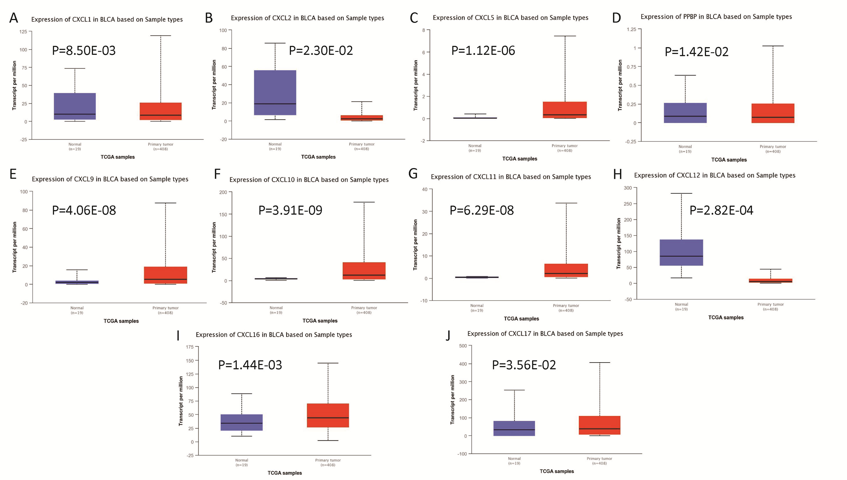
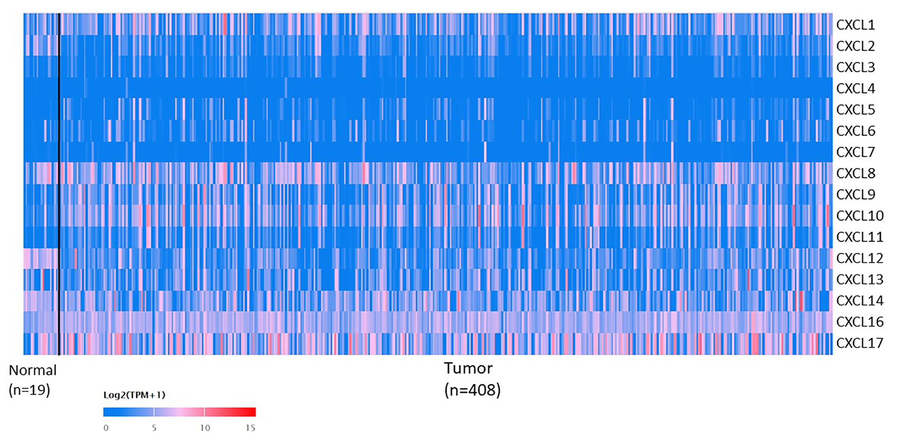
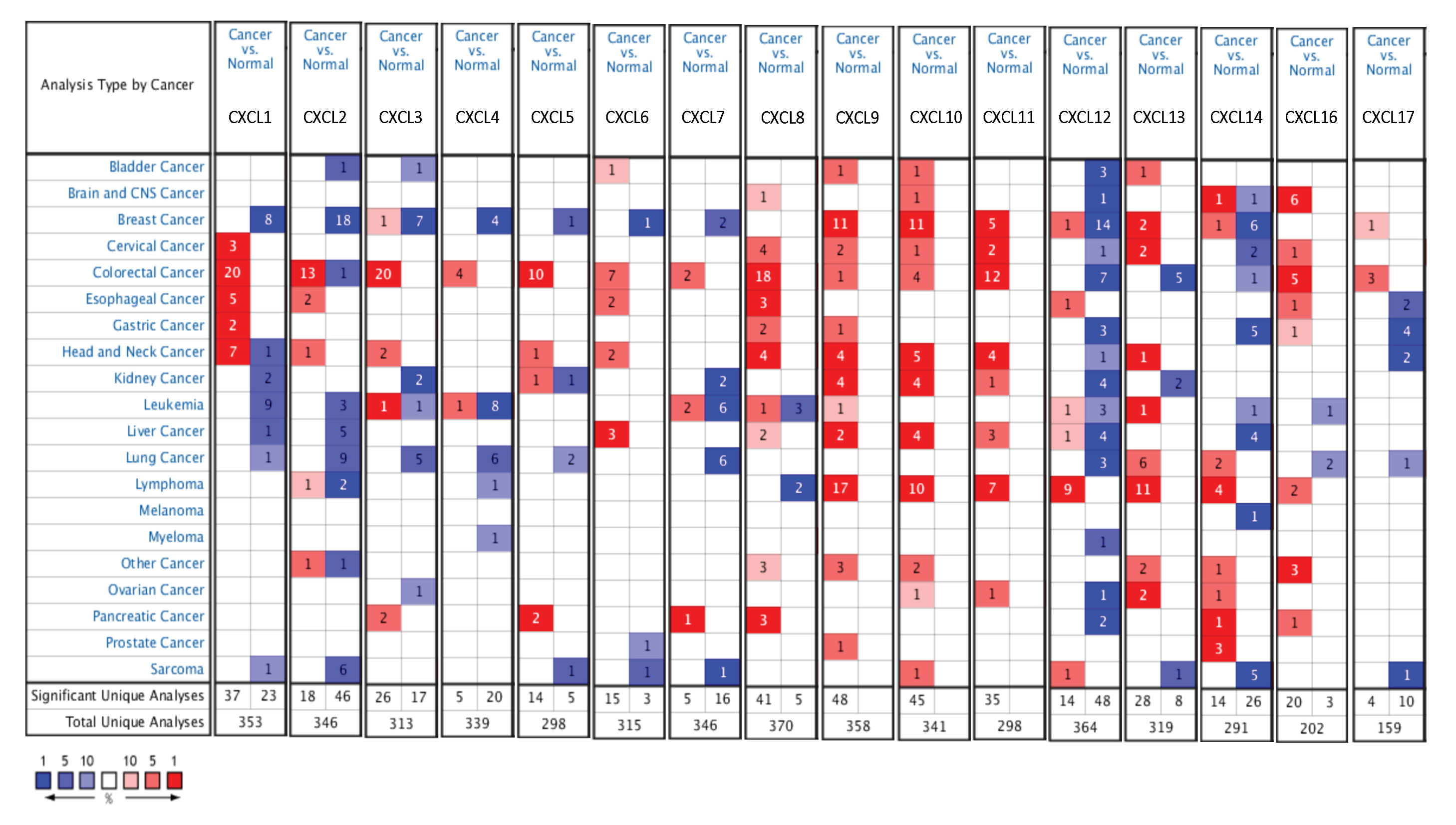
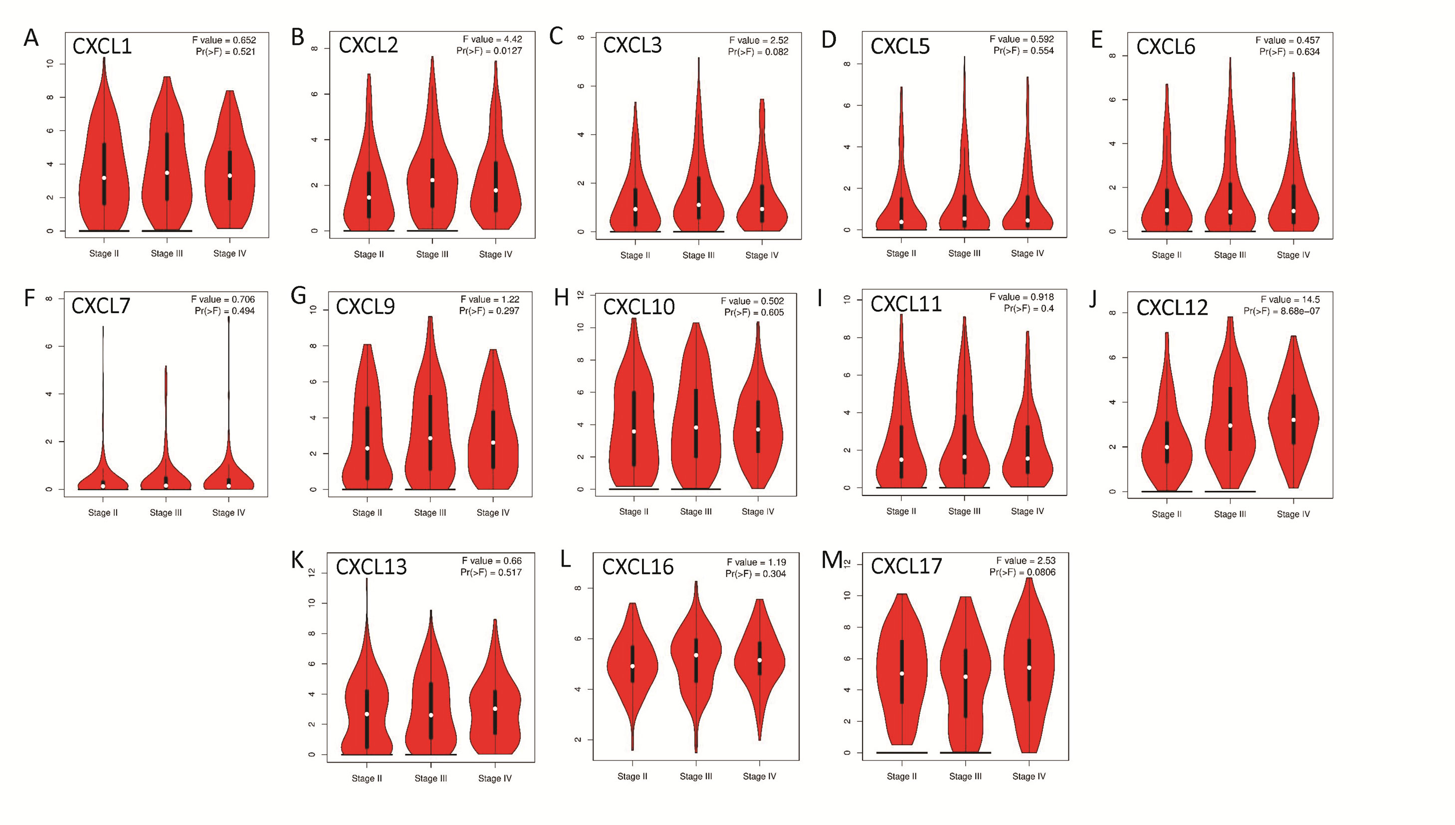
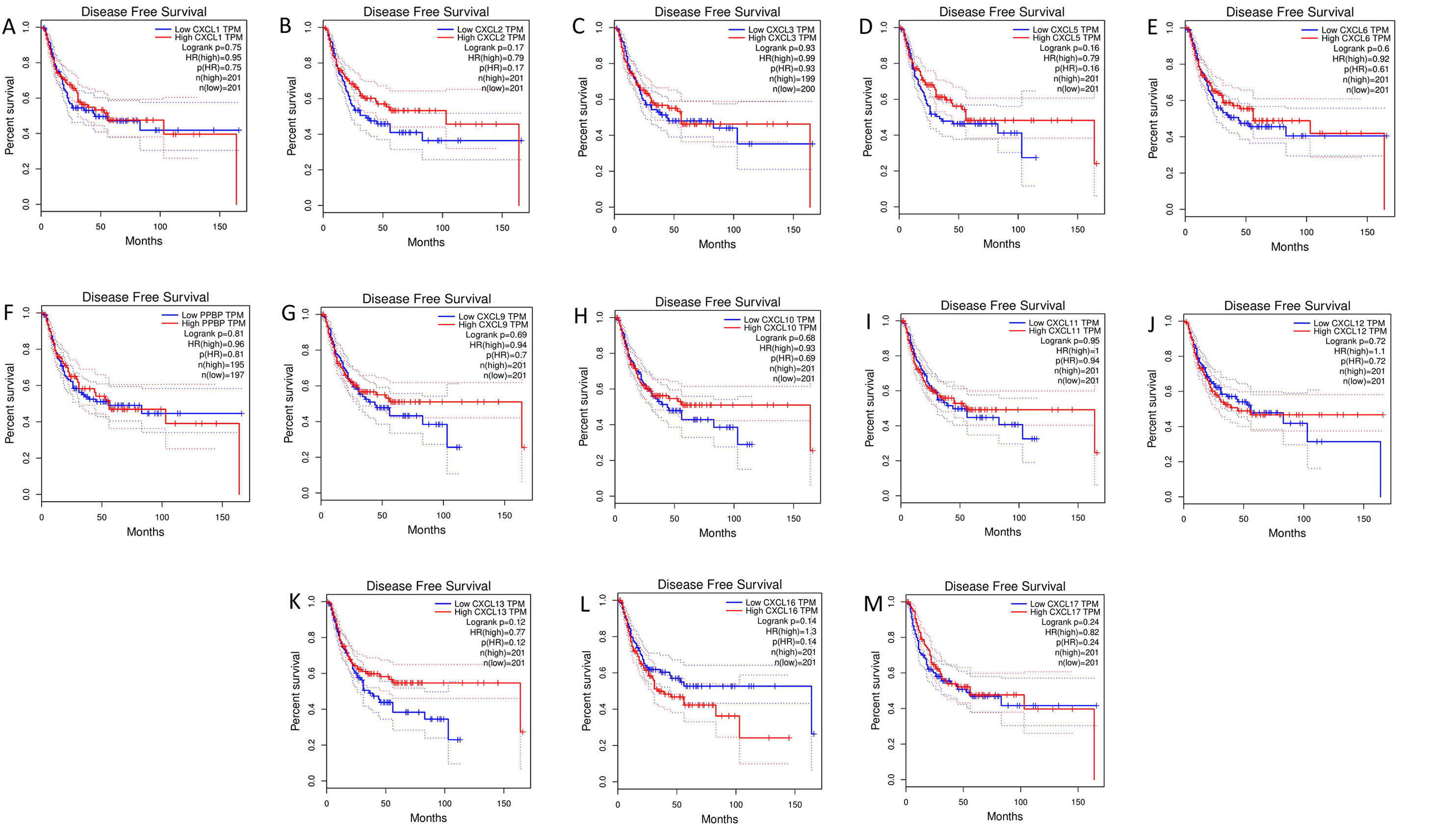
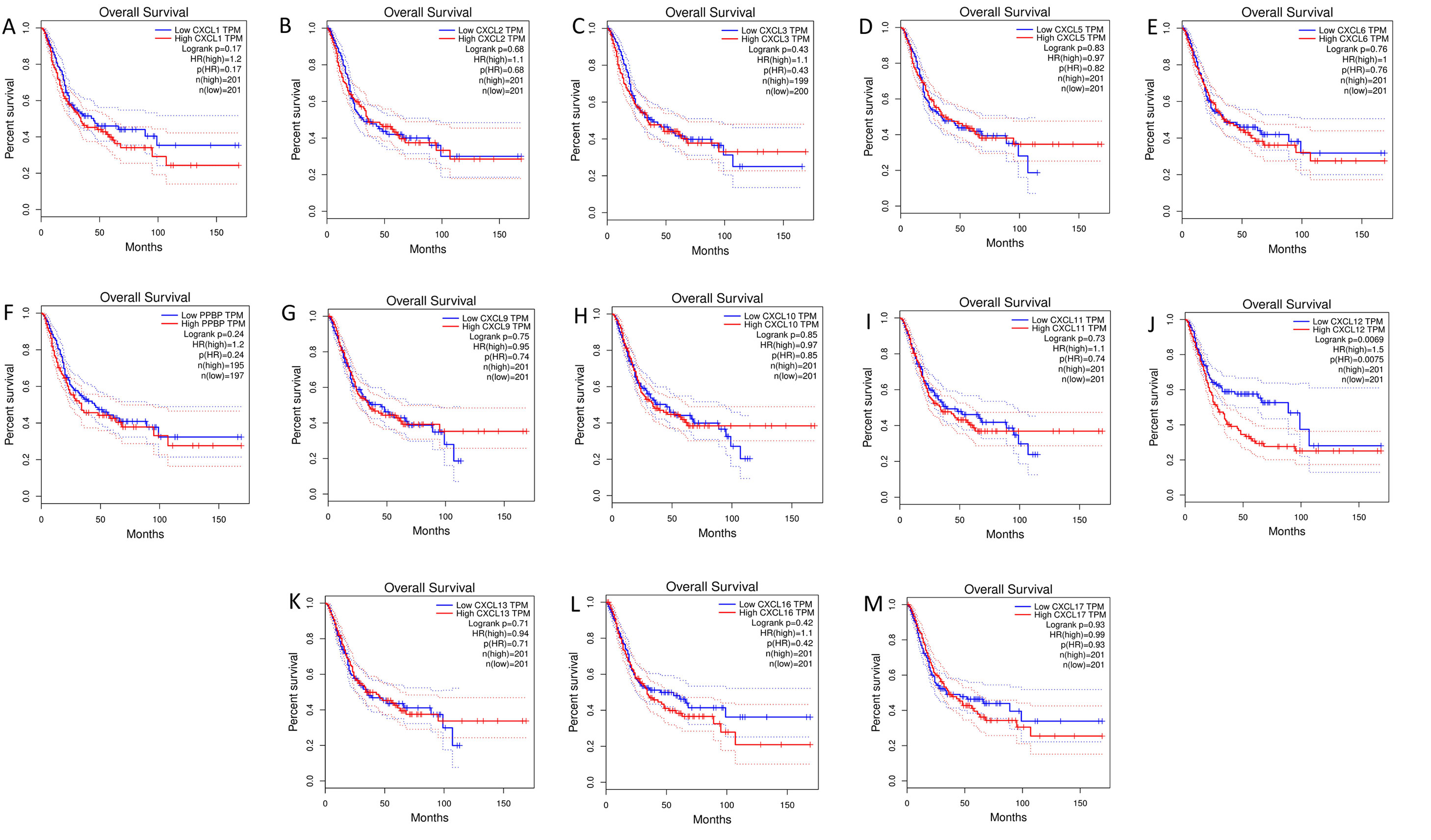
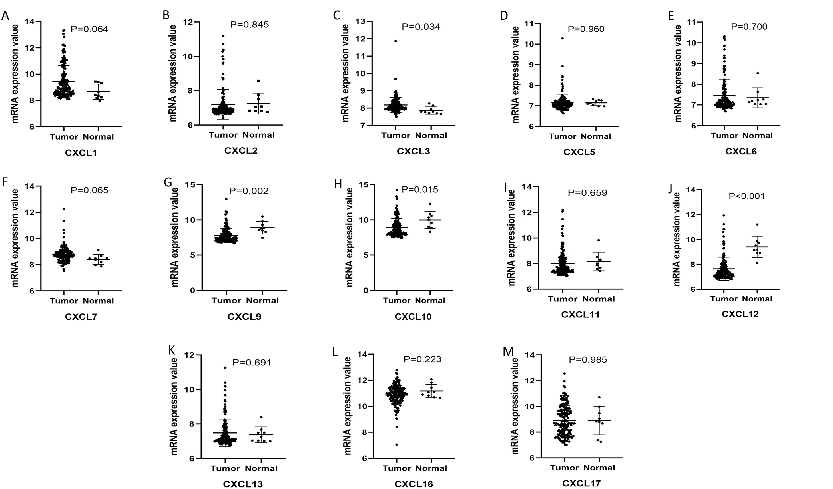
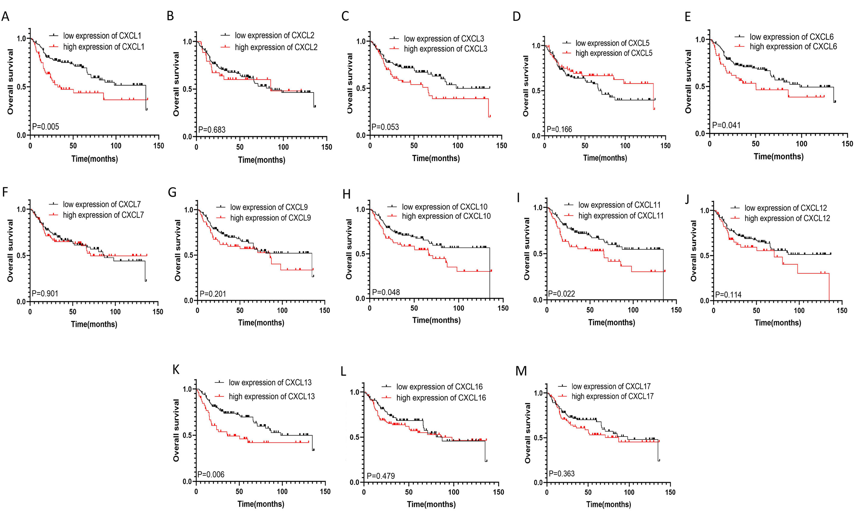
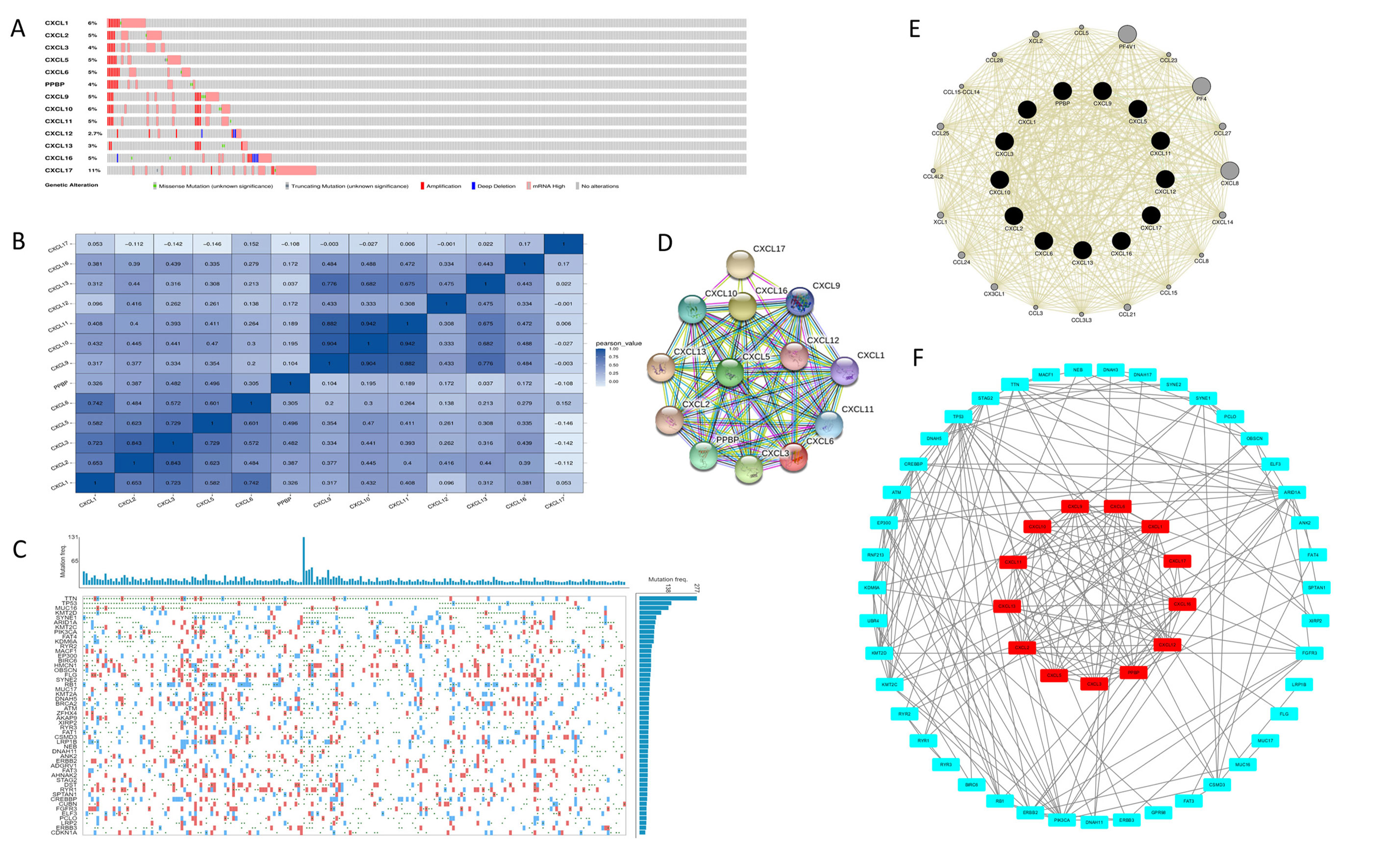
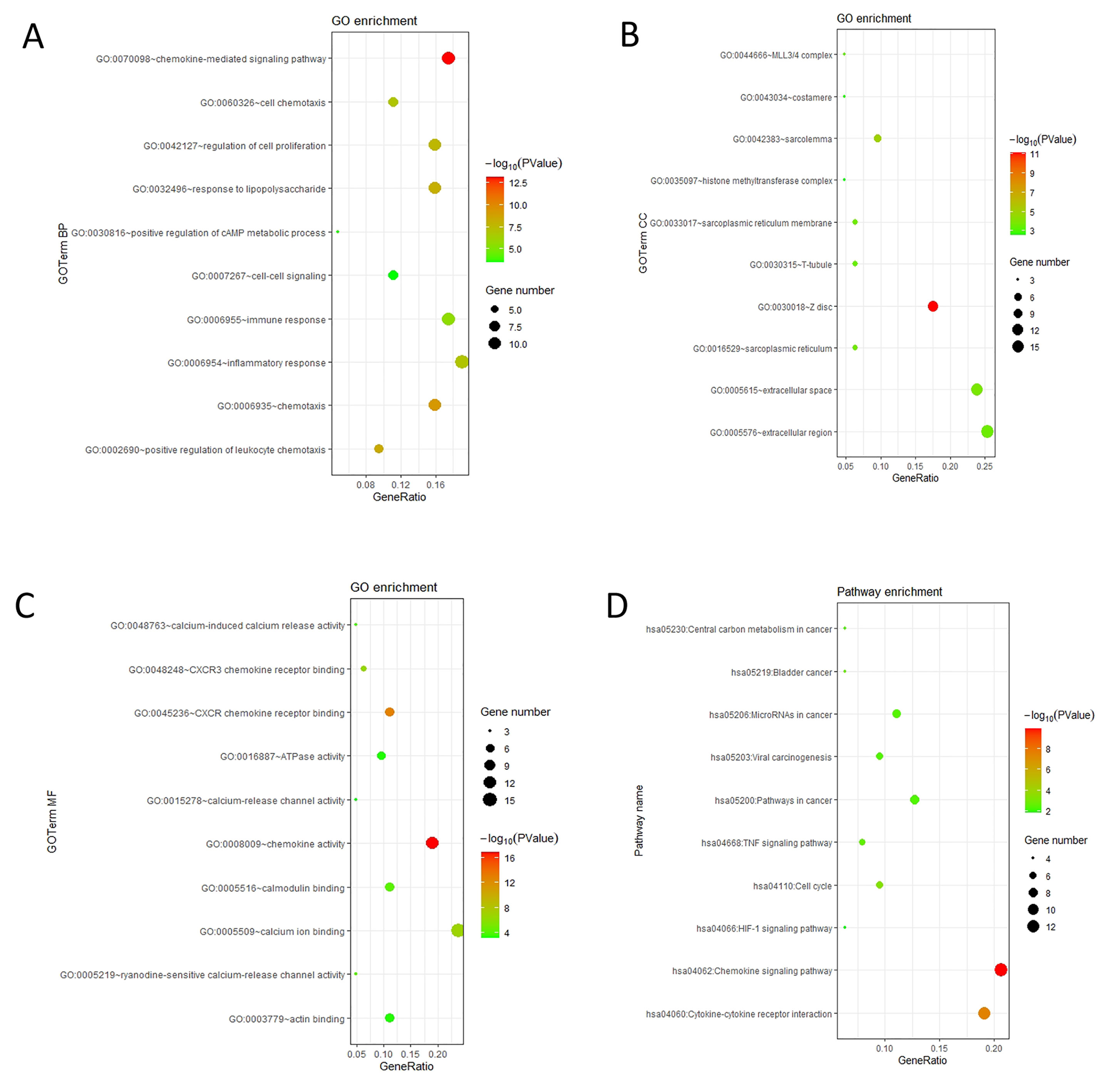
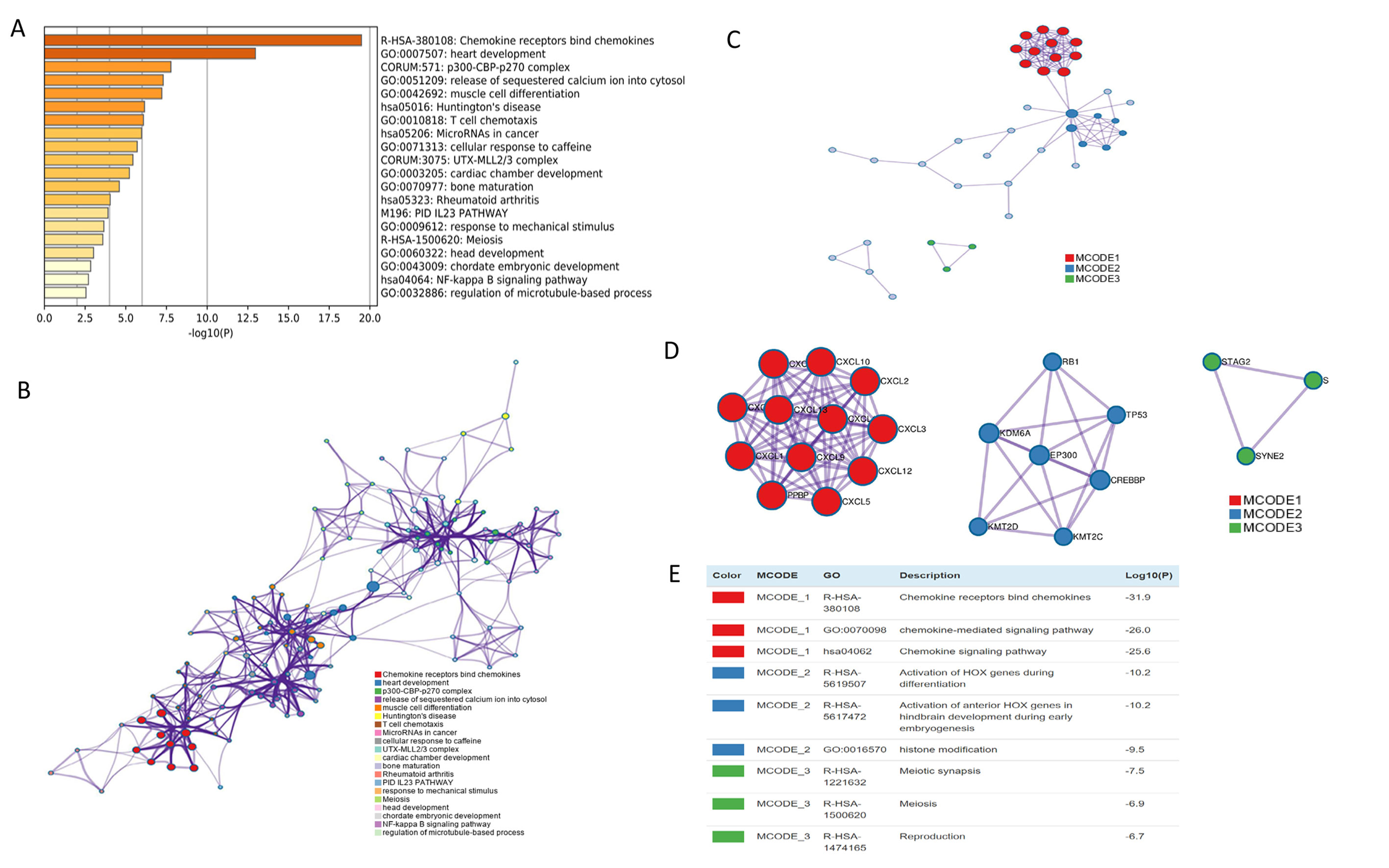
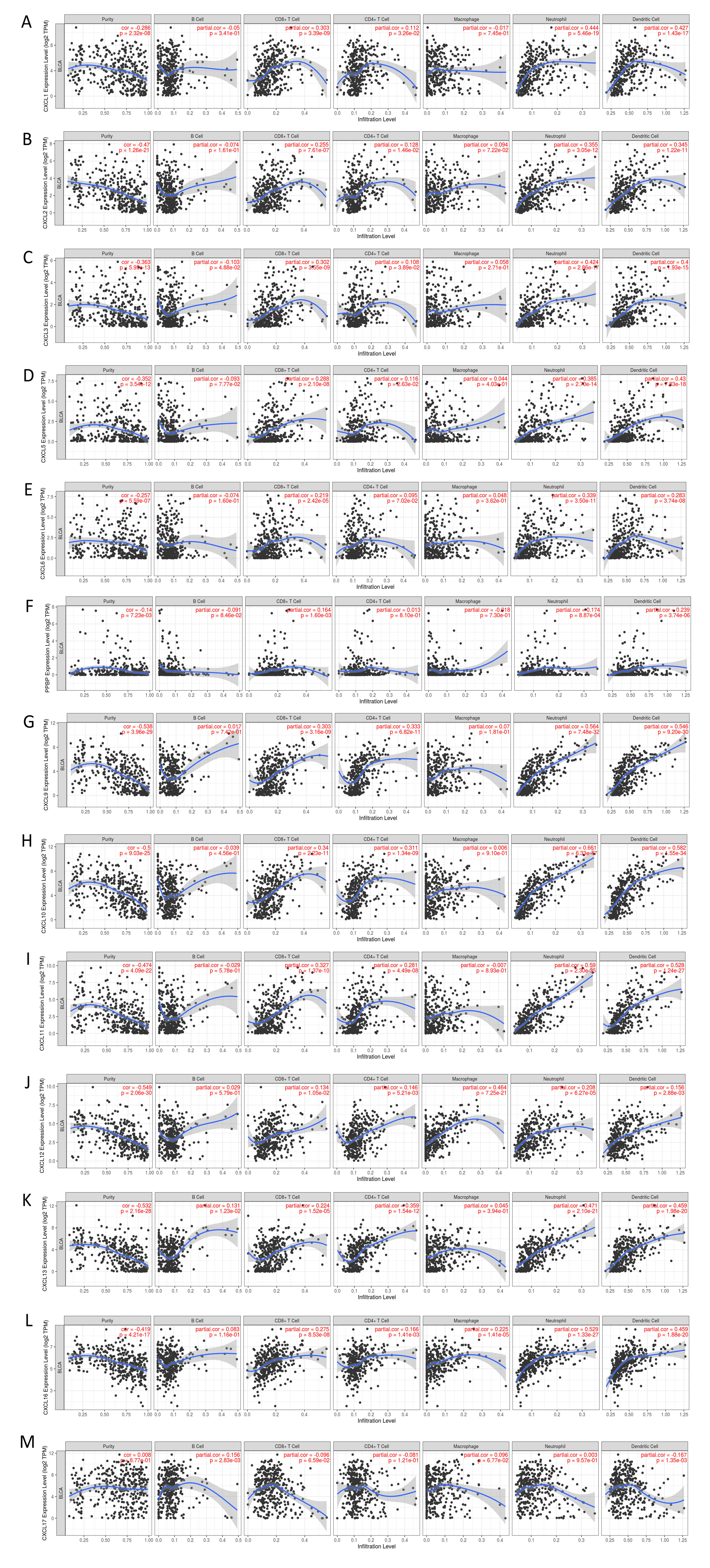
The mRNA levels of C-X-C motif chemokine ligand (CXCL)1, CXCL5, CXCL6, CXCL7, CXCL9, CXCL10, CXCL11, CXCL13, CXCL16, and CXCL17 were increased significantly increased, and those of CXCL2, CXCL3, and CXCL12 were decreased significantly in BLCA tissues as assessed using the Oncomine, TCGA, and GEO databases. GEO showed that high levels of CXCL1, CXCL6, CXCL10, CXCL11, and CXCL13 mRNA expression are associated significantly with the poor overall survival (all p < 0.05), and similarly, those of CXCL2 and CXCL12 in the TCGA database (p < 0.05). The predominant signaling pathways involving the differentially expressed CXC chemokines are cell cycle, chemokine, and cytokine-cytokine receptor interaction. Moreover, transcription factors such as Sp1 transcription factor (SP1), nuclear factor kappa B subunit 1 (NFKB1), and RELA proto-oncogene, NF-KB subunit (RELA) were likely play critical roles in regulating CXC chemokine expression. LYN proto-oncogene, src family tyrosine kinase (LYN) and LCK proto-oncogene, src family tyrosine kinase (LCK) were identified as the key targets of these CXC chemokines. MicroRNAs miR200 and miR30 were identified as the main microRNAs that interact with several CXC chemokines through an miRNA-target network. The expression of these chemokines is closely associated with the infiltration of six categories of immune cells.

Conclusion
We explored the CXC chemokines superfamily-based biomarkers associated with BLCA prognosis using public databases, and provided possible chemokine targets for patients with BLCA.
- bladder cancer,
- biomarkers,
- CXC chemokines,
- microenvironment
Citation: Xiaoqi Sun, Qunxi Chen, Lihong Zhang, Jiewei Chen, Xinke Zhang. Exploration of prognostic biomarkers and therapeutic targets in the microenvironment of bladder cancer based on CXC chemokines[J]. Mathematical Biosciences and Engineering, 2021, 18(5): 6262-6287. doi: 10.3934/mbe.2021313

Related Papers:

Abstract

Background

Bladder cancer (BLCA) has a high rate of morbidity and mortality, and is considered as one of the most malignant tumors of the urinary system. Tumor cells interact with surrounding interstitial cells, playing a key role in carcinogenesis and progression, which is partly mediated by chemokines. CXC chemokines exert anti-tumor biological roles in the tumor microenvironment and affect patient prognosis. Nevertheless, their expression and prognostic values patients with BLCA remain unclear.

Methods

We used online tools, including Oncomine, UALCAN, GEPIA, GEO databases, cBioPortal, GeneMANIA, DAVID 6.8, Metascape, TRUST (version 2.0), LinkedOmics, TCGA, and TIMER2.0 to perform the relevant analysis.

Results

The mRNA levels of C-X-C motif chemokine ligand (CXCL)1, CXCL5, CXCL6, CXCL7, CXCL9, CXCL10, CXCL11, CXCL13, CXCL16, and CXCL17 were increased significantly increased, and those of CXCL2, CXCL3, and CXCL12 were decreased significantly in BLCA tissues as assessed using the Oncomine, TCGA, and GEO databases. GEO showed that high levels of CXCL1, CXCL6, CXCL10, CXCL11, and CXCL13 mRNA expression are associated significantly with the poor overall survival (all p < 0.05), and similarly, those of CXCL2 and CXCL12 in the TCGA database (p < 0.05). The predominant signaling pathways involving the differentially expressed CXC chemokines are cell cycle, chemokine, and cytokine-cytokine receptor interaction. Moreover, transcription factors such as Sp1 transcription factor (SP1), nuclear factor kappa B subunit 1 (NFKB1), and RELA proto-oncogene, NF-KB subunit (RELA) were likely play critical roles in regulating CXC chemokine expression. LYN proto-oncogene, src family tyrosine kinase (LYN) and LCK proto-oncogene, src family tyrosine kinase (LCK) were identified as the key targets of these CXC chemokines. MicroRNAs miR200 and miR30 were identified as the main microRNAs that interact with several CXC chemokines through an miRNA-target network. The expression of these chemokines is closely associated with the infiltration of six categories of immune cells.

Conclusion

We explored the CXC chemokines superfamily-based biomarkers associated with BLCA prognosis using public databases, and provided possible chemokine targets for patients with BLCA.

References

[1]	S. Antoni, J. Ferlay, I. Soerjomataram, A. Znaor, A. Jemal, F. Bray, Bladder cancer incidence and mortality: a global overview and recent trends, Eur. Urol., 71 (2017), 96-108. doi: 10.1016/j.eururo.2016.06.010
[2]	J. Ferlay, I. Soerjomataram, R. Dikshit, S. Eser, C. Mathers, M. Rebelo, et al., Cancer incidence and mortality worldwide: sources, methods and major patterns in GLOBOCAN 2012, Int. J. Cancer, 136 (2015), E359-E386.
[3]	International Collaboration of Trialists, International phase Ⅲ trial assessing neoadjuvant cisplatin, methotrexate, and vinblastine chemotherapy for muscle-invasive bladder cancer: long-term results of the BA06 30894 trial, J. Clin. Oncol., 29 (2011), 2171-2177.
[4]	Bladder cancer: diagnosis and management of bladder cancer: (c) NICE (2015) Bladder cancer: diagnosis and management of bladder cancer, BJU Int., 120 (2017), 755-765.
[5]	D. H. Aggen, C. G. Drake, Biomarkers for immunotherapy in bladder cancer: a moving target, J. Immunother. Cancer, 5 (2017), 94.
[6]	M. Babjuk, M. Burger, E. M. Comperat, P. Gontero, A. H. Mostafid, J. Palou, et al., European association of urology guidelines on non-muscle-invasive bladder cancer (TaT1 and carcinoma in situ) - 2019 update, Eur. Urol., 76 (2019), 639-657.
[7]	S. Cambier, R. J. Sylvester, L. Collette, P. Gontero, M. A. Brausi, G. van Andel, et al., EORTC nomograms and risk groups for predicting recurrence, progression, and disease-specific and overall survival in non-muscle-invasive stage Ta-T1 urothelial bladder cancer patients treated with 1-3 years of maintenance bacillus calmette-guerin, Eur. Urol., 69 (2016), 60-69.
[8]	R. Dutta, A. Abdelhalim, J. W. Martin, S. L. Vernez, B. Faltas, Y. Lotan, et al., Effect of tumor location on survival in urinary bladder adenocarcinoma: a population-based analysis, Urol. Oncol., 34 (2016), 531.e1-531.e6.
[9]	S. Wu, X. Zhao, Y. Wang, Z. Zhong, L. Zhang, J. Cao, et al., Pretreatment neutrophil-lymphocyte ratio as a predictor in bladder cancer and metastatic or unresectable urothelial carcinoma patients: a pooled analysis of comparative studies, Cell. Physiol. Biochem., 46 (2018), 1352-1364
[10]	E. Ojerholm, A. Smith, W. T. Hwang, B. C. Baumann, K. N. Tucker, S. P. Lerner, et al., Neutrophil-to-lymphocyte ratio as a bladder cancer biomarker: Assessing prognostic and predictive value in SWOG 8710, Cancer, 123 (2017), 794-801.
[11]	A. Kamoun, A. de Reynies, Y. Allory, G. Sjodahl, A. G. Robertson, R. Seiler, et al., A consensus molecular classification of muscle-invasive bladder cancer, Eur. Urol., 77 (2020), 420-433.
[12]	J. A. Witjes, H. M. Bruins, R. Cathomas, E. M. Comperat, N. C. Cowan, G. Gakis, et al., European association of urology guidelines on muscle-invasive and metastatic bladder cancer: summary of the 2020 guidelines, Eur. Urol., 79 (2021) 82-104,
[13]	P. A. Gerber, A. Hippe, B. A. Buhren, A. Muller, B. Homey, Chemokines in tumor-associated angiogenesis, Biol. Chem., 390 (2009), 1213-1223.
[14]	E. C. Keeley, B. Mehrad, R. M. Strieter, CXC chemokines in cancer angiogenesis and metastases, Adv. Cancer Res., 106 (2010), 91-111. doi: 10.1016/S0065-230X(10)06003-3
[15]	A. D. Luster, Chemokines--chemotactic cytokines that mediate inflammation, N. Engl. J. Med., 338 (1998), 436-445. doi: 10.1056/NEJM199802123380706
[16]	S. Struyf, P. Proost, J. Van Damme, Regulation of the immune response by the interaction of chemokines and proteases, Adv. Immunol., 81 (2003), 1-44. doi: 10.1016/S0065-2776(03)81001-5
[17]	E. C. Keeley, B. Mehrad, R. M. Strieter, Chemokines as mediators of neovascularization, Arterioscler. Thromb. Vasc. Biol., 28 (2008), 1928-1936. doi: 10.1161/ATVBAHA.108.162925
[18]	A. Muller, B. Homey, H. Soto, N. Ge, D. Catron, M. E. Buchanan, et al., Involvement of chemokine receptors in breast cancer metastasis, Nature, 410 (2001), 50-56.
[19]	F. Bertolini, C. Dell'Agnola, P. Mancuso, C. Rabascio, A. Burlini, S. Monestiroli, et al., CXCR4 neutralization, a novel therapeutic approach for non-Hodgkin's lymphoma, Cancer Res., 62 (2002), 3106-3112.
[20]	J. B. Rubin, A. L. Kung, R. S. Klein, J. A. Chan, Y. Sun, K. Schmidt, et al., A small-molecule antagonist of CXCR4 inhibits intracranial growth of primary brain tumors, Proc. Natl. Acad. Sci. U S A, 100 (2003), 13513-13518.
[21]	J. Vandercappellen, J. Van Damme, S. Struyf, The role of CXC chemokines and their receptors in cancer, Cancer Lett., 267 (2008), 226-244. doi: 10.1016/j.canlet.2008.04.050
[22]	M. Miyake, S. Hori, Y. Morizawa, Y. Tatsumi, Y. Nakai, S. Anai, et al., CXCL1-mediated interaction of cancer cells with tumor-associated macrophages and cancer-associated fibroblasts promotes tumor progression in human bladder cancer, Neoplasia, 18 (2016), 636-646.
[23]	A. Nazari, H. Khorramdelazad, G. Hassanshahi, Biological/pathological functions of the CXCL12/CXCR4/CXCR7 axes in the pathogenesis of bladder cancer, Int. J. Clin. Oncol., 22 (2017), 991-1000. doi: 10.1007/s10147-017-1187-x
[24]	H. Zhang, Y. L. Ye, M. X. Li, S. B. Ye, W. R. Huang, T. T. Cai, et al., CXCL2/MIF-CXCR2 signaling promotes the recruitment of myeloid-derived suppressor cells and is correlated with prognosis in bladder cancer, Oncogene, 36 (2017), 2095-2104.
[25]	A. Nazari, Z. Ahmadi, G. Hassanshahi, M. Abbasifard, Z. Taghipour, S. K. Falahati-Pour, et al., Effective treatments for bladder cancer affecting CXCL9/CXCL10/CXCL11/CXCR3 axis: a review, Oman Med. J., 35 (2020), e103.
[26]	J. Zheng, X. Zhu, J. Zhang, CXCL5 knockdown expression inhibits human bladder cancer T24 cells proliferation and migration, Biochem. Biophys. Res. Commun., 446 (2014), 18-24. doi: 10.1016/j.bbrc.2014.01.172
[27]	D. R. Rhodes, J. Yu, K. Shanker, N. Deshpande, R. Varambally, D. Ghosh, et al., ONCOMINE: a cancer microarray database and integrated data-mining platform, Neoplasia, 6 (2004), 1-6.
[28]	D. S. Chandrashekar, B. Bashel, S. A. H. Balasubramanya, C. J. Creighton, I. Ponce-Rodriguez, B. Chakravarthi, et al., UALCAN: a portal for facilitating tumor subgroup gene expression and survival analyses, Neoplasia, 19 (2017), 649-658.
[29]	Z. Tang, C. Li, B. Kang, G. Gao, C. Li, Z. Zhang, GEPIA: a web server for cancer and normal gene expression profiling and interactive analyses, Nucleic. Acids. Res., 45 (2017), W98-W102.
[30]	J. Gao, B. A. Aksoy, U. Dogrusoz, G. Dresdner, B. Gross, S. O. Sumer, et al., Integrative analysis of complex cancer genomics and clinical profiles using the cBioPortal, Sci. Signal., 6 (2013), pl1.
[31]	D. Warde-Farley, S. L. Donaldson, O. Comes, K. Zuberi, R. Badrawi, P. Chao, et al., The GeneMANIA prediction server: biological network integration for gene prioritization and predicting gene function, Nucleic Acids Res., 38 (2010), W214-220.
[32]	D. Szklarczyk, A. L. Gable, D. Lyon, A. Junge, S. Wyder, J. Huerta-Cepas, et al., STRING v11: protein-protein association networks with increased coverage, supporting functional discovery in genome-wide experimental datasets, Nucleic Acids Res., 47 (2019), D607-D613.
[33]	W. Huang da, B. T. Sherman, R. A. Lempicki, Systematic and integrative analysis of large gene lists using DAVID bioinformatics resources, Nat. Protoc., 4 (2009), 44-57. doi: 10.1038/nprot.2008.211
[34]	Y. Zhou, B. Zhou, L. Pache, M. Chang, A. H. Khodabakhshi, O. Tanaseichuk, et al., Metascape provides a biologist-oriented resource for the analysis of systems-level datasets, Nat. Commun., 10 (2019), 1-10.
[35]	H. Han, J. W. Cho, S. Lee, A. Yun, H. Kim, D. Bae, et al., TRRUST v2: an expanded reference database of human and mouse transcriptional regulatory interactions, Nucleic Acids Res., 46 (2018), D380-D386.
[36]	T. Li, J. Fu, Z. Zeng, D. Cohen, J. Li, Q. Chen, et al., TIMER2.0 for analysis of tumor-infiltrating immune cells, Nucleic Acids Res., 48 (2020), W509-W514.
[37]	S. V. Vasaikar, P. Straub, J. Wang, B. Zhang, LinkedOmics: analyzing multi-omics data within and across 32 cancer types, Nucleic Acids Res., 46 (2018), D956-D963.
[38]	M. Sanchez-Carbayo, N. D. Socci, J. Lozano, F. Saint, C. Cordon-Cardo, Defining molecular profiles of poor outcome in patients with invasive bladder cancer using oligonucleotide microarrays, J. Clin. Oncol., 24 (2006), 778-789. doi: 10.1200/JCO.2005.03.2375
[39]	J. S. Lee, S. H. Leem, S. Y. Lee, S. C. Kim, E. S. Park, S. B. Kim, et al., Expression signature of E2F1 and its associated genes predict superficial to invasive progression of bladder tumors, J. Clin. Oncol., 28 (2010), 2660-2667.
[40]	M. S. Lawrence, P. Stojanov, P. Polak, G. V. Kryukov, K. Cibulskis, A. Sivachenko, et al., Mutational heterogeneity in cancer and the search for new cancer-associated genes, Nature, 499 (2013), 214-218.
[41]	K. H. Susek, M. Karvouni, E. Alici, A. Lundqvist, The role of CXC chemokine receptors 1-4 on immune cells in the tumor microenvironment, Front. Immunol., 9 (2018), 2159.
[42]	V. Mollica Poeta, M. Massara, A. Capucetti, R. Bonecchi, chemokines and chemokine receptors: new targets for cancer immunotherapy, Front. Immunol., 10 (2019), 379.
[43]	A. F. Schott, L. J. Goldstein, M. Cristofanilli, P. A. Ruffini, S. McCanna, J. M. Reuben, et al., Phase Ib pilot study to evaluate reparixin in combination with weekly paclitaxel in patients with HER-2-negative metastatic breast cancer, Clin. Cancer Res., 23 (2017), 5358-5365.
[44]	T. M. Nywening, A. Wang-Gillam, D. E. Sanford, B. A. Belt, R. Z. Panni, B. M. Cusworth, et al., Targeting tumour-associated macrophages with CCR2 inhibition in combination with FOLFIRINOX in patients with borderline resectable and locally advanced pancreatic cancer: a single-centre, open-label, dose-finding, non-randomised, phase 1b trial, Lancet Oncol., 17 (2016), 651-662.
[45]	C. Berlato, M. N. Khan, T. Schioppa, R. Thompson, E. Maniati, A. Montfort, et al., A CCR4 antagonist reverses the tumor-promoting microenvironment of renal cancer, J. Clin. Invest., 127 (2017), 801-813.
[46]	D. Di Mitri, A. Toso, J. J. Chen, M. Sarti, S. Pinton, T. R. Jost, et al., Tumour-infiltrating Gr-1+ myeloid cells antagonize senescence in cancer, Nature, 515 (2014), 134-137.
[47]	C. Wang, A. Li, S. Yang, R. Qiao, X. Zhu, J. Zhang, CXCL5 promotes mitomycin C resistance in non-muscle invasive bladder cancer by activating EMT and NF-kappaB pathway, Biochem. Biophys. Res. Commun., 498 (2018), 862-868. doi: 10.1016/j.bbrc.2018.03.071
[48]	I. Bieche, C. Chavey, C. Andrieu, M. Busson, S. Vacher, L. Le Corre, et al., CXC chemokines located in the 4q21 region are up-regulated in breast cancer, Endocr. Relat. Cancer, 14 (2007), 1039-1052.
[49]	X. R. Yang, K. Brown, M. T. Landi, P. Ghiorzo, C. Badenas, M. Xu, et al., Duplication of CXC chemokine genes on chromosome 4q13 in a melanoma-prone family, Pigment Cell Melanoma Res., 25 (2012), 243-247.
[50]	M. Lusti-Narasimhan, C. A. Power, B. Allet, S. Alouani, K. B. Bacon, J. J. Mermod, et al., Mutation of Leu25 and Val27 introduces CC chemokine activity into interleukin-8, J. Biol. Chem., 270 (1995), 2716-2721.
[51]	S. Y. Lim, A. E. Yuzhalin, A. N. Gordon-Weeks, R. J. Muschel, Targeting the CCL2-CCR2 signaling axis in cancer metastasis, Oncotarget, 7 (2016), 28697-28710. doi: 10.18632/oncotarget.7376
[52]	P. J. Sarvaiya, D. Guo, I. Ulasov, P. Gabikian, M. S. Lesniak, Chemokines in tumor progression and metastasis, Oncotarget, 4 (2013), 2171-2185. doi: 10.18632/oncotarget.1426
[53]	F. C. Kischkel, D. A. Lawrence, A. Tinel, H. LeBlanc, A. Virmani, P. Schow, et al., Death receptor recruitment of endogenous caspase-10 and apoptosis initiation in the absence of caspase-8, J. Biol. Chem., 276 (2001), 46639-46646.
[54]	X. Chen, J. J. Subleski, H. Kopf, O. M. Howard, D. N. Mannel, J. J. Oppenheim, Cutting edge: expression of TNFR2 defines a maximally suppressive subset of mouse CD4+CD25+FoxP3+ T regulatory cells: applicability to tumor-infiltrating T regulatory cells, J. Immunol., 180 (2008), 6467-6471. doi: 10.4049/jimmunol.180.10.6467
[55]	T. Tanaka, T. Imamura, M. Yoneda, A. Irie, H. Ogi, M. Nagata, et al., Enhancement of active MMP release and invasive activity of lymph node metastatic tongue cancer cells by elevated signaling via the TNF-alpha-TNFR1-NF-kappaB pathway and a possible involvement of angiopoietin-like 4 in lung metastasis, Int. J. Oncol., 49 (2016), 1377-1384.
[56]	Y. Guo, Y. Feng, H. Liu, S. Luo, J. W. Clarke, P. G. Moorman, et al., Potentially functional genetic variants in the TNF/TNFR signaling pathway genes predict survival of patients with non-small cell lung cancer in the PLCO cancer screening trial, Mol. Carcinog., 58 (2019), 1094-1104.
[57]	I. Zidi, S. Mestiri, A. Bartegi, N. B. Amor, TNF-alpha and its inhibitors in cancer, Med. Oncol., 27 (2010), 185-198.
[58]	X. Yuan, A. Gajan, Q. Chu, H. Xiong, K. Wu, G. S. Wu, Developing TRAIL/TRAIL death receptor-based cancer therapies, Cancer Metastasis Rev., 37 (2018), 733-748. doi: 10.1007/s10555-018-9728-y
[59]	S. Biswas, S. Roy Chowdhury, G. Mandal, S. Purohit, A. Gupta, A. Bhattacharyya, RelA driven co-expression of CXCL13 and CXCR5 is governed by a multifaceted transcriptional program regulating breast cancer progression, Biochim. Biophys. Acta Mol. Basis Dis., 1865 (2019), 502-511. doi: 10.1016/j.bbadis.2018.12.002
[60]	B. S. Kochupurakkal, Z. C. Wang, T. Hua, A. C. Culhane, S. J. Rodig, K. Rajkovic-Molek, et al., RelA-induced interferon response negatively regulates proliferation, PLoS One, 10 (2015), e0140243.
[61]	M. Lesina, S. M. Wormann, J. Morton, K. N. Diakopoulos, O. Korneeva, M. Wimmer, et al., RelA regulates CXCL1/CXCR2-dependent oncogene-induced senescence in murine Kras-driven pancreatic carcinogenesis, J. Clin. Invest., 126 (2016), 2919-2932.
[62]	E. Ronin, M. Lubrano di Ricco, R. Vallion, J. Divoux, H. K. Kwon, S. Gregoire, et al., The NF-kappaB RelA transcription factor is critical for regulatory T cell activation and stability, Front. Immunol., 10 (2019), 2487.
[63]	X. Qu, J. Han, Y. Zhang, X. Wang, H. Fan, F. Hua, et al., TLR4-RelA-miR-30a signal pathway regulates Th17 differentiation during experimental autoimmune encephalomyelitis development, J. Neuroinflammation, 16 (2019), 1-13.
[64]	J. Concetti, C. L. Wilson, NFKB1 and cancer: friend or foe?, Cells, 7 (2018), 133.
[65]	P. Li, J. Gu, X. Yang, H. Cai, J. Tao, X. Yang, et al., Functional promoter -94 ins/del ATTG polymorphism in NFKB1 gene is associated with bladder cancer risk in a Chinese population, PLoS One, 8 (2013), e71604.
[66]	R. Roskoski Jr., Src protein-tyrosine kinase structure and regulation, Biochem. Biophys. Res. Commun., 324 (2004), 1155-1164.
[67]	V. B. Venkadakrishnan, A. D. DePriest, S. Kumari, D. Senapati, S. Ben-Salem, Y. Su, et al., Protein Kinase N1 control of androgen-responsive serum response factor action provides rationale for novel prostate cancer treatment strategy, Oncogene, 38 (2019), 4496-4511.
[68]	A. Franko, M. Kovarova, S. Feil, R. Feil, R. Wagner, M. Heni, et al., cGMP-dependent protein kinase I (cGKI) modulates human hepatic stellate cell activation, Metabolism, 88 (2018), 22-30.
[69]	F. Schuler, S. Afreen, C. Manzl, G. Hacker, M. Erlacher, A. Villunger, Checkpoint kinase 1 is essential for fetal and adult hematopoiesis, EMBO Rep., 20 (2019), e47026.
[70]	D. D. Browning, I. K. Kwon, R. Wang, cGMP-dependent protein kinases as potential targets for colon cancer prevention and treatment, Future Med. Chem., 2 (2010), 65-80. doi: 10.4155/fmc.09.142
[71]	W. Lin, S. Chen, Checkpoint Kinase 1 Is Overexpressed during HPV16-Induced Cervical Carcinogenesis, Gynecol. Obstet. Invest., 83 (2018), 299-305. doi: 10.1159/000487943
[72]	J. M. Lamar, Y. Xiao, E. Norton, Z. G. Jiang, G. M. Gerhard, S. Kooner, et al., SRC tyrosine kinase activates the YAP/TAZ axis and thereby drives tumor growth and metastasis, J. Biol. Chem., 294 (2019), 2302-2317.
[73]	L. Mao, S. Liu, L. Hu, L. Jia, H. Wang, M. Guo, et al., miR-30 family: a promising regulator in development and disease, Biomed. Res. Int., 2018 (2018), 9623412.
[74]	H. Yin, Y. Wang, Y. Wu, X. Zhang, X. Zhang, J. Liu, et al., EZH2-mediated Epigenetic Silencing of miR-29/miR-30 targets LOXL4 and contributes to tumorigenesis, metastasis, and immune microenvironment remodeling in breast cancer, Theranostics, 10 (2020), 8494-8512.
[75]	S. Jiang, D. Miao, M. Wang, J. Lv, Y. Wang, J. Tong, MiR-30-5p suppresses cell chemoresistance and stemness in colorectal cancer through USP22/Wnt/beta-catenin signaling axis, J. Cell. Mol. Med., 23 (2019), 630-640. doi: 10.1111/jcmm.13968
[76]	B. Farhood, M. Najafi, K. Mortezaee, CD8(+) cytotoxic T lymphocytes in cancer immunotherapy: a review, J. Cell. Physiol., 234 (2019), 8509-8521.
[77]	R. M. Bremnes, L. T. Busund, T. L. Kilvaer, S. Andersen, E. Richardsen, E. E. Paulsen, et al., The role of tumor-infiltrating lymphocytes in development, progression, and prognosis of non-small cell lung cancer, J. Thorac. Oncol., 11 (2016), 789-800.

Reader Comments

Your name:*

Email:*
© 2021 the Author(s), licensee AIMS Press. This is an open access article distributed under the terms of the Creative Commons Attribution License (http://creativecommons.org/licenses/by/4.0)