A nonstandard finite difference scheme for the SVICDR model to predict COVID-19 dynamics

Sarah Treibert; Helmut Brunner; Matthias Ehrhardt; Sarah Treibert; Helmut Brunner; Matthias Ehrhardt

doi:10.3934/mbe.2022056

Mathematical Biosciences and Engineering

2022, Volume 19, Issue 2: 1213-1238. doi: 10.3934/mbe.2022056

Previous Article Next Article

Research article Special Issues

A nonstandard finite difference scheme for the SVICDR model to predict COVID-19 dynamics

1.
Chair of Applied Mathematics and Numerical Analysis, School of Mathematics and Natural Sciences, University of Wuppertal, Wuppertal 42119, Germany
2.
Chair of Health Economics, Faculty of Management and Economics, University of Wuppertal, Wuppertal 42119, Germany

Academic Editor: Salihu S. Musa

Received: 15 September 2021 Accepted: 27 October 2021 Published: 01 December 2021

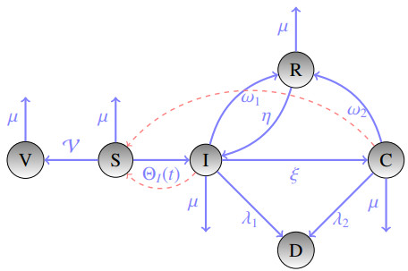
In the context of 2019 coronavirus disease (COVID-19), considerable attention has been paid to mathematical models for predicting country- or region-specific future pandemic developments. In this work, we developed an SVICDR model that includes a susceptible, an all-or-nothing vaccinated, an infected, an intensive care, a deceased, and a recovered compartment. It is based on the susceptible-infectious-recovered (SIR) model of Kermack and McKendrick, which is based on ordinary differential equations (ODEs). The main objective is to show the impact of parameter boundary modifications on the predicted incidence rate, taking into account recent data on Germany in the pandemic, an exponential increasing vaccination rate in the considered time window and trigonometric contact and quarantine rate functions. For the numerical solution of the ODE systems a model-specific non-standard finite difference (NSFD) scheme is designed, that preserves the positivity of solutions and yields the correct asymptotic behaviour.
- nonstandard finite difference scheme,
- COVID-19,
- SARS-CoV-2,
- compartment models,
- epidemiology
Citation: Sarah Treibert, Helmut Brunner, Matthias Ehrhardt. A nonstandard finite difference scheme for the SVICDR model to predict COVID-19 dynamics[J]. Mathematical Biosciences and Engineering, 2022, 19(2): 1213-1238. doi: 10.3934/mbe.2022056

Related Papers:

Abstract

In the context of 2019 coronavirus disease (COVID-19), considerable attention has been paid to mathematical models for predicting country- or region-specific future pandemic developments. In this work, we developed an SVICDR model that includes a susceptible, an all-or-nothing vaccinated, an infected, an intensive care, a deceased, and a recovered compartment. It is based on the susceptible-infectious-recovered (SIR) model of Kermack and McKendrick, which is based on ordinary differential equations (ODEs). The main objective is to show the impact of parameter boundary modifications on the predicted incidence rate, taking into account recent data on Germany in the pandemic, an exponential increasing vaccination rate in the considered time window and trigonometric contact and quarantine rate functions. For the numerical solution of the ODE systems a model-specific non-standard finite difference (NSFD) scheme is designed, that preserves the positivity of solutions and yields the correct asymptotic behaviour.

References

[1]	World Health Organization, WHO-convened Global Study of Origins of SARS-CoV-2: China Part, Joint WHO-China Study, Joint Report, 2021. Available from: http://www.ecns.cn/m/news/society/2021-03-15/detail-ihainwmv2680654.shtml.
[2]	C. M. Freuling, A. Breithaupt, T. Müller, J. Sehl, A. Balkema-Buschmann, M. Rissmann, et al., Susceptibility of raccoon dogs for experimental SARS-CoV-2 infection, Emerg. Infect. Dis. J., 26 (2020), 2982–2985. doi: 10.3201/eid2612.203733. doi: 10.3201/eid2612.203733
[3]	World Health Organization, Origins of SARS-CoV-2, 2021. Available from: https://apps.who.int/iris/bitstream/handle/10665/332197/WHO-2019-nCoV-FAQ-Virus_origin-2020.1-eng.pdf.
[4]	European Centre for Disease Prevention and Control, 2021. Available from: https://www.ecdc.europa.eu/en/geographical-distribution-2019-ncov-cases.
[5]	L. Bretschger, E. Grieg, P. J. J. Welfens, T. Xiong, COVID-19 infections and fatalities developments: empirical evidence for OECD countries and newly industrialized economies, Inter. Economics Economic Policy, 17 (2020), 801–147. doi: 10.1007/s10368-020-00487-x. doi: 10.1007/s10368-020-00487-x
[6]	S. Bugalia, V. P. Bajiya, J. P. Tripathi, M. T. Li, G. Q. Sun, Mathematical modeling of COVID-19 transmission: the roles of intervention strategies and lockdown, Math. Biosci. Engrg., 17 (2020), 5961–5986. doi: 10.3934/mbe.2020318. doi: 10.3934/mbe.2020318
[7]	John Hopkins University, 2021. Available from: https://coronavirus.jhu.edu/vaccines/international.
[8]	O. Diekmann, J. A. P. Heesterbeek, M. G. Roberts, The construction of next-generation matrices for compartmental epidemic models, J. Royal Soc. Interface, 7 (2009), 873–885. doi: 10.1098/rsif.2009.0386. doi: 10.1098/rsif.2009.0386
[9]	Z. Abreu, G. Cantin, C. J. Silva, Analysis of a COVID-19 compartmental model: a mathematical and computational approach, Math. Biosci. Engrg., 18 (2021), 7979–7998. doi:10.3934/mbe.2021396. doi: 10.3934/mbe.2021396
[10]	M. Martcheva, An introduction to mathematical epidemiology, Springer, (2015), 10–13.
[11]	Robert Koch-Institute, The methodological glossary provides explanations on concepts and definitions from epidemiology and health reporting, 2021. Available from: https://www.rki.de/DE/Content/Gesundheitsmonitoring/Gesundheitsberichterstattung/Glossar/g-be_glossar_catalog.html?cms_lv2=36862902.
[12]	O.N. Bjornstad, Epidemics, Springer, (2018), 32.
[13]	Robert Koch-Institute, Epidemiologischer steckbrief zu SARS-CoV-2 und COVID-19, 2021. Available from: https://www.rki.de/DE/Content/InfAZ/N/Neuartiges_Coronavirus/Steckbrief.html.
[14]	F. Ball, D. Sirl, Evaluation of vaccination strategies for SIR epidemics on random networks incorporating household structure, J. Math. Biol., 76 (2018), 483–530. doi: 10.1007/s00285-017-1139-0. doi: 10.1007/s00285-017-1139-0
[15]	S. Treibert, Mathematical Modelling and Nonstandard Schemes for the Corona Virus Pandemic, Master Thesis, University of Wuppertal, 2021.
[16]	R. Wölfel, V. M. Corman, W. Guggemos, M. Seilmaier, S. Zange, M. A. Müller, et al., Virological assessment of hospitalized patients with COVID-2019, Nature, 581 (2020), 465–469. doi: 10.1038/s41586-020-2196-x. doi: 10.1038/s41586-020-2196-x
[17]	X. He, E. H. Y. Lau, P. Wu, X. L. Deng, J. Wang, X. X. Hao, et al., Temporal dynamics in viral shedding and transmissibility of COVID-19, Nat. Med., 26 (2020), 672–675. doi: 10.1101/2020.03.15.20036707. doi: 10.1101/2020.03.15.20036707
[18]	C. A. Walsh, K. Jordan, B. Clyne, D. Rohde, L. Rohde, P. Byrne, et al., SARS-CoV-2 detection, viral load and infectivity over the course of an infection, J. Infection, 81 (2020), 357–371. doi: 10.1016/j.jinf.2020.06.067. doi: 10.1016/j.jinf.2020.06.067
[19]	W. S. Hart, P. K. Maini, R. N. Thompson, High infectiousness immediately before COVID-19 symptom onset highlights the importance of continued contact tracing, eLife, 10 (2021), e65534. doi: 10.10.7554/elife.65534. doi: 10.10.7554/elife.65534
[20]	O. Diekmann, W. F. de Graaf, M. E. E. Kretzschmar, P. F. M. Teunis, Waning and boosting: on the dynamics of immune status, J. Math. Biol., 77 (2018), 2023–2048. doi: 10.1007/s00285-018-1239-5. doi: 10.1007/s00285-018-1239-5
[21]	S. F. Lumley, D. O'Donell, N. E. Stoesser, P. C. Matthews, A. Howarth, S. B. Hatch, et al., Antibody status and incidence of SARS-CoV-2 infection in health care workers, New England J. Med., 384 (2020), 533–540. doi: 10.1056/NEJMoa2034545. doi: 10.1056/NEJMoa2034545
[22]	X. Wang, Studying social awareness of physical distancing in mitigating COVID-19 transmission, Math. Biosci. Engrg., 17 (2020), 7428-7441. doi: 10.3934/mbe.2020380. doi: 10.3934/mbe.2020380
[23]	A. Perasso, An introduction to the basic reproduction number in mathematical epidemiology, Esaim-Proc. Surveys, 62 (2018), 123–138. doi: 10.1051/proc/201862123. doi: 10.1051/proc/201862123
[24]	M. V. Barbarossa, N. Bogya, A. Dénes, G. Röst, H. V. Varma, Z. Vizi, Fleeing lockdown and its impact on the size of epidemic outbreaks in the source and target regions–a COVID-19 lesson, Nature Sci. Rep., 9233 (2021), 9233. doi: 10.21203/rs.3.rs-82993/v1. doi: 10.21203/rs.3.rs-82993/v1
[25]	N. Chintis, J. M. Cushing, J. M. Hyman, Determining important parameters in the spread of malaria through the sensitivity analysis of a mathematical model, Bull. Math. Biology, 70 (2008), 1272–1296. doi: 10.1007/s11538-008-9299-0. doi: 10.1007/s11538-008-9299-0
[26]	R. Wilkinson, F. Ball, K. Sharkey, The relationships between message passing, pairwise, Kermack–McKendrick and stochastic SIR epidemic models, J. Math. Biol., 75 (2017), 1563–1590. doi: 10.1007/s00285-017-1123-8. doi: 10.1007/s00285-017-1123-8
[27]	R. E. Mickens, Applications of nonstandard finite difference schemes, World Scientific, (2000).
[28]	A. Suryanto, A conservative nonstandard finite difference scheme for SIR epidemic model, in International Conferences and Workshops on Basic and Applied Sciences, (2011). doi: 10.1063/1.5004277.
[29]	M. Ehrhardt, R. E. Mickens, A nonstandard finite difference scheme for solving a Zika Virus Model, Forthcoming.
[30]	Robert Koch-Institute, COVID-19-Fälle nach Altersgruppe und Meldewoche, 2021. Available from: https://www.rki.de/DE/Content/InfAZ/N/Neuartiges_Coronavirus/Daten/Altersverteilung.html.
[31]	Robert Koch-Institute, Todesfälle nach Sterbedatum, 2021. Available from: https://www.rki.de/DE/Content/InfAZ/N/Neuartiges_Coronavirus/Projekte_RKI/COVID-19_Todesfaelle.html.
[32]	German Interdisciplinary Association for Intensive and Emergency Medicine, Anzahl der Corona-Patienten (COVID-19) in intensivmedizinischer Behandlung in Deutschland seit März 2020, 2021. Available from: https://de.statista.com/statistik/daten/studie/1181959/umfrage/intensivmedizinische-behandlungen-von-corona-patienten-in-deutschland/.
[33]	COVID-19 vaccination dashboard, 2021. Available from: https://impfdashboard.de/daten.
[34]	S. Treibert, Matlab scripts, Available from: https://git.uni-wuppertal.de/1449563/covid-19-modelling/-/tree/master/NSFD_Paper_2021.
[35]	Robert Koch-Institute, Bericht zu Virusvarianten von SARS-CoV-2 in Deutschland, 2021. Available from: https://www.rki.de/DE/Content/InfAZ/N/Neuartiges_Coronavirus/DESH/Bericht_VO-C_2021-06-30.pdf?_blob=publicationFile
[36]	M. Ehrhardt, J. Gašper, S. Kilianová, SIR-based mathematical modeling of infectious diseases with vaccination and waning immunity, J. Comput. Sci., 7 (2019), 101027. doi: 10.1016/j.jocs.2019.101027. doi: 10.1016/j.jocs.2019.101027

Reader Comments

Your name:*

Email:*
© 2022 the Author(s), licensee AIMS Press. This is an open access article distributed under the terms of the Creative Commons Attribution License (http://creativecommons.org/licenses/by/4.0)