Processing math: 84%
Research article

A system dynamics approach to biodiesel fund management in Indonesia

  • Received: 18 August 2020 Accepted: 29 October 2020 Published: 09 November 2020
  • Indonesia, which is strongly supportive of renewable energy development, meets its obligation to extensively employ renewable energy through the mandatory mixing of palm oil-derived biodiesel with diesel, a fossil fuel. The success of the program is inseparable from the government's provision of incentives which involve paying the difference in cost between biodiesel and diesel through export taxes collected from producers of palm oil and its derivatives. However, the increase in the government's mandatory target is not in line with the higher revenue obtained with the result that under current policy conditions the government will not be able to provide incentives for the B30 plan during the next few years. This research presents a dynamic simulation modelling of Indonesia's biodiesel program and analyzes the policy applied in support of that program. A system dynamics model is proposed to enable decision-makers to understand the relationship between the different variables inherent in the system and the impact of different variables on the continuity of the biodiesel program in Indonesia. The system dynamics model consists of three sub-models: the palm oil production sub-model, the biodiesel demand and production sub-model and the biodiesel fund management sub-model. Fund management of biodiesel is specifically discussed, starting with the source of funds, through fund management, to the impact of fund availability on the biodiesel mandatory program's continuity. The simulation shows that increasing palm oil production capacity is insufficient in order to ensure the success of the government program. Simulations indicate that the biodiesel program will operate optimally if two prerequisites are satisfied; first, that the levy policy adopted is not dependent upon crude palm oil (CPO) prices and, second, that the provision of incentives is limited solely to those required by the prevailing Public Service Obligation (PSO).

    Citation: Fitriani Tupa R. Silalahi, Togar M. Simatupang, Manahan P. Siallagan. A system dynamics approach to biodiesel fund management in Indonesia[J]. AIMS Energy, 2020, 8(6): 1173-1198. doi: 10.3934/energy.2020.6.1173

    Related Papers:

    [1] Ruimin Wu, Yinsheng Jiang, Liyuan Wang . Gradient estimates in generalized Orlicz spaces for quasilinear elliptic equations via extrapolation. AIMS Mathematics, 2023, 8(10): 24153-24161. doi: 10.3934/math.20231231
    [2] Ru Bai, Tiantian Chen, Sen Liu . Global stability solution of the 2D incompressible anisotropic magneto-micropolar fluid equations. AIMS Mathematics, 2022, 7(12): 20627-20644. doi: 10.3934/math.20221131
    [3] Abdul Mateen, Ghulam Hussain Tipu, Loredana Ciurdariu, Fengping Yao . Analytical soliton solutions of the Kairat-Ⅱ equation using the Kumar–Malik and extended hyperbolic function methods. AIMS Mathematics, 2025, 10(4): 8721-8752. doi: 10.3934/math.2025400
    [4] Ye Xue, Yongzhen Ge, Yunlan Wei . The existence of a nontrivial solution to an elliptic equation with critical Sobolev exponent and a general potential well. AIMS Mathematics, 2025, 10(3): 7339-7354. doi: 10.3934/math.2025336
    [5] Khaled Kefi, Nasser S. Albalawi . Three weak solutions for degenerate weighted quasilinear elliptic equations with indefinite weights and variable exponents. AIMS Mathematics, 2025, 10(2): 4492-4503. doi: 10.3934/math.2025207
    [6] Xingang Zhang, Zhe Liu, Ling Ding, Bo Tang . Global solutions to a nonlinear Fokker-Planck equation. AIMS Mathematics, 2023, 8(7): 16115-16126. doi: 10.3934/math.2023822
    [7] Nafissa Toureche Trouba, Mohamed E. M. Alngar, Reham M. A. Shohib, Haitham A. Mahmoud, Yakup Yildirim, Huiying Xu, Xinzhong Zhu . Novel solitary wave solutions of the (3+1)–dimensional nonlinear Schrödinger equation with generalized Kudryashov self–phase modulation. AIMS Mathematics, 2025, 10(2): 4374-4411. doi: 10.3934/math.2025202
    [8] F. A. Mohammed, Mohammed K. Elboree . Soliton solutions and periodic solutions for two models arises in mathematical physics. AIMS Mathematics, 2022, 7(3): 4439-4458. doi: 10.3934/math.2022247
    [9] Shuai Li, Tianqing An, Weichun Bu . Existence results for Schrödinger type double phase variable exponent problems with convection term in RN. AIMS Mathematics, 2024, 9(4): 8610-8629. doi: 10.3934/math.2024417
    [10] Ugur G. Abdulla . Generalized Newton-Leibniz formula and the embedding of the Sobolev functions with dominating mixed smoothness into Hölder spaces. AIMS Mathematics, 2023, 8(9): 20700-20717. doi: 10.3934/math.20231055
  • Indonesia, which is strongly supportive of renewable energy development, meets its obligation to extensively employ renewable energy through the mandatory mixing of palm oil-derived biodiesel with diesel, a fossil fuel. The success of the program is inseparable from the government's provision of incentives which involve paying the difference in cost between biodiesel and diesel through export taxes collected from producers of palm oil and its derivatives. However, the increase in the government's mandatory target is not in line with the higher revenue obtained with the result that under current policy conditions the government will not be able to provide incentives for the B30 plan during the next few years. This research presents a dynamic simulation modelling of Indonesia's biodiesel program and analyzes the policy applied in support of that program. A system dynamics model is proposed to enable decision-makers to understand the relationship between the different variables inherent in the system and the impact of different variables on the continuity of the biodiesel program in Indonesia. The system dynamics model consists of three sub-models: the palm oil production sub-model, the biodiesel demand and production sub-model and the biodiesel fund management sub-model. Fund management of biodiesel is specifically discussed, starting with the source of funds, through fund management, to the impact of fund availability on the biodiesel mandatory program's continuity. The simulation shows that increasing palm oil production capacity is insufficient in order to ensure the success of the government program. Simulations indicate that the biodiesel program will operate optimally if two prerequisites are satisfied; first, that the levy policy adopted is not dependent upon crude palm oil (CPO) prices and, second, that the provision of incentives is limited solely to those required by the prevailing Public Service Obligation (PSO).


    This article deals with the nonlinear elliptic equation with measure data of the type

    divA(x,u)=μin Ω. (1.1)

    Here ΩRn (n2) is a bounded domain, the unknown uW1,P(Ω) with an N-function P() which will be introduced in Section 2, and A(x,u)L1loc(Ω,Rn). In (1.1), μ is a Radon measure defined on Ω with finite total mass |μ|(Ω)<. Moreover, if the measure μ is actually an L1-function, then

    |μ|(Q):=Q|μ(x)|dx (1.2)

    for a measurable subset QΩ. We assume that measure μ satisfies the following condition:

    (M) There exists some θ0(0,n1) such that

    |μ|(B(x0,2R))(2R)θ0 (1.3)

    holds for all x0Ω and every R>0.

    In this article, we assume that the Carathéodory vector field A:Ω×RnRn is C1-regular in the gradient variable ξ, and satisfies A(x,0)=0, and the growth, ellipticity, and continuity conditions, i.e., there are constants 0s1, 0<νL, and K1 such that

    (A1) {|A(x,ξ)|+|Aξ(x,ξ)|(|ξ|2+s2)12LP((|ξ|2+s2)12)(|ξ|2+s2)12,ν1P(|ξ2ξ1|)A(x,ξ2)A(x,ξ1),ξ2ξ1,|A(x,ξ)A(y,ξ)|Kω(|xy|)P((|ξ|2+s2)12)(|ξ|2+s2)12

    for any x,yΩ and ξ,ξ1,ξ2Rn. In (A1), the function ω:[0,)[0,) has the following hypothesis.

    (A2)ωis a non-decreasing concave function such thatω(0)=limρ0ω(ρ)=0andω()1.

    Moreover, ω is assumed to satisfy the Dini-continuous condition:

    (A3)  d(R):=R0ω(ρ)dρρ<

    for every 0<R1.

    A significant example of (1.1) is the p-Laplacian type equation, for which s=0, p(1,), P(x)=xp, and A(u)=|u|p2u. Then Eq (1.1) can be expressed as

    div(|u|p2u)=μ.

    The relevant research on the regularities of solutions to elliptic equations starts with Kilpeläinen and Malý [1,2], and extends with a different technique by Trudinger and Wang [3]. Later, Duzaar and Mingione make a further study in [4]. Those results show a standard fact that solutions to non-homogeneous p-Laplacian-type equations with measure data can be pointwise estimated in a natural way by involving the classical nonlinear Wolff potential Wμβ,p(x,R) [5], that is,

    Wμβ,p(x,R):=R0(|μ|(B(x,ρ))ρnβp)1p1dρρ,β(0,np].

    Based on the relationship between Wolff potential and Riesz potential, Mingione et al. [6,7] find out pointwise gradient estimates hold for general quasilinear degenerate equations by applying the Riesz potential

    Iμβ(x,R):=Wμβ2,2(x,R)=R0|μ|(B(x,ρ))ρnβdρρ,β>0. (1.4)

    Baroni proves pointwise gradient bounds for solutions in terms of linear Riesz potentials in [8]. In addition, the caloric Riesz potential serves as a means for pointwise estimation of the spatial gradient of solutions to nonlinear degenerate parabolic equations [9].

    Further, pointwise gradient estimates via the nonlinear Wolff potentials for weak solutions to various quasilinear elliptic equations with measure data are obtained by Mingione [10] and Yao [11]. More generally, pointwise potential estimates for elliptic equations and systems with Orlicz growth are studied in [12,13,14], respectively.

    In recent years, a great deal of effort has gone into investigating nonlinear elliptic equations and systems involving measure data. Chilebicka et al. [15] study estimates including precise continuity and Hölder continuity criteria by the means of potential of a Wolff type; they also provide regularity estimates of the solutions and their gradients in the generalized Marcinkiewicz scale [16]. The existence of solutions in the framework of renormalized solutions is introduced in [17]. There are many interesting results in [18,19,20].

    In this article, a weak solution to (1.1) is a function uW1,P(Ω) such that

    ΩA(x,u),φdζ=Ωφdμ, (1.5)

    whenever φC0(Ω). Inspired by Mingione et al. [4,10,21], the main objective is to present pointwise potential estimates and interior Hölder continuity of weak solutions to (1.1) by using (1.4) in the Sobolev-Orlicz spaces.

    We state our pointwise estimates in Theorems 1.1 and 1.2. It is important to note that θ0 in the following theorems will be introduced in (1.3). The first main result is the gradient pointwise estimates of u as follows.

    Theorem 1.1. Let uC1(Ω)W1,P(Ω) be a weak solution to (1.1) under the assumptions (A1), (A2), (A3), Radon measure μ satisfy μL1(Ω) and (M), and P be an N-function with Δ2(P,˜P)< satisfying Assumption 2.4 and (2.12). There exists a constant CC(n,ν,L,K,s,θ0,CΔ2,C1)>0 and a positive radius ˜R<1 such that the pointwise estimate

    P(|u(x0)|)CB(x0,R)[P(|u|)+P(s)]dx+CIμnθ0(x0,4R) (1.6)

    holds whenever B(x0,R)Ω and 0<R˜R. In (1.6), denotes integral average, Δ2-condition, CΔ2, and C1 will be described in Definition 2.3 and Lemma 2.5, respectively.

    On the basis of Theorem 1.1, we demonstrate the pointwise estimate of u.

    Theorem 1.2. Let uC0(Ω)W1,P(Ω) be a weak solution to (1.1) under the assumptions (A1)1, (A1)2, Radon measure μ satisfy μL1(Ω) and (M), and P be an N-function with Δ2(P,˜P)< satisfying Assumption 2.4, and (2.12). There exists a constant CC(n,ν,L,θ0,CΔ2,C1,diam(Ω))>0 and a positive radius R<1 such that for every rR the pointwise estimate

    P(|u(x0)|)Cr1+ε0B(x0,r)P(|u|r)dx+CrαIμnθ0α(x0,2r) (1.7)

    holds, where ε0 and α will be introduced in Lemmas 2.5 and 3.3, respectively.

    Inspired by Mingione's result [10], the following theorem expounds the Hölder continuity of the solution u.

    Theorem 1.3 (Interior Hölder type estimate). Let uC0(Ω)W1,P(Ω) be a weak solution to (1.1) under the assumptions (A1), (A2), let μ be a Radon measure satisfying μL1(Ω) and (M), and let P be an N-function satisfying Δ2(P,˜P)<, Assumption 2.4, and (2.12). Then there exists constants α[0,1) and 0<R<1 such that for every x,yB(x0,2R)Ω, there holds

    P(|u(x)u(y)|)C[Iμnθ0α(x,2R)+Iμnθ0α(y,2R)+B(x0,2R)P(|u|R)dζ+P(s)]|xy|α,

    where the constant C depends on n,ν,L,θ0,ω(),CΔ2,C1, and diam(Ω).

    Remark 1.4. Drawing upon the Riesz potential, our results present pointwise estimates and Hölder continuity within the more generalized framework of Sobolev-Orlicz spaces. Notably, (1.6) provides an estimate of u, whereas (1.7) estimates u itself. We shall leverage Lemma 2.11 to relate u to u.

    In this article, we adopt several technical tools and methods in Sobolev-Orlicz spaces, and explore the properties of solutions of homogeneous equations to those of inhomogeneous equations with measure data. We first establish Proposition 3.2, which reveals the density of the Riesz potential and serves as a crucial conclusion in facilitating the proof of subsequent comparison lemmas. The proof of the comparison estimate is divided into two intricate steps; the first step requires Sobolev-type embedding, while the second primarily employs scaling changes. Our primary objective is to prove pointwise potential estimates and Hölder continuity, which is shown essentially by oscillation estimates of solutions. By utilizing summation methods and involving the Riesz potential, we proceed from deriving the estimates of the gradient of u to those of u itself. Ultimately, we employ the sharp maximal functions, and achieve the interior Hölder estimates of solutions.

    This article is organized as follows: In Section 2, we state fundamental tools and definitions such as N-functions and maximal functions. Section 3 is devoted to the proof of Lemmas 3.4 and 3.9, and Section 4 presents supporting results, to gather Caccioppoli-type inequality and maximal estimate towards the proof of the main theorems. In the last section, we present the proofs of Theorems 1.1–1.3, respectively.

    In this section, we give the definitions and tools of N-functions, function spaces; classical inequalities, and maximal functions.

    The following definitions and results are standard in the context of N-function; see [22].

    Definition 2.1. A function P:[0,)[0,) is said to be an N-function, if P is convex, differentiable, and its derivative P is a right continuous, non-decreasing function satisfying that P(0)=0 and P(t)>0 for t>0.

    Definition 2.2. The complementary function ˜P:[0,)[0,) is defined by

    ˜P(x)=supt0[xtP(t)].

    Definition 2.3. We say that P satisfied the Δ2-condition, if there exists CΔ2>0 such that

    P(2t)CΔ2P(t)

    for all t0. By Δ2(P) we denote the smallest constant CΔ2. The function P is said to satisfy the 2-condition, if ˜PΔ2. Then we define

    Δ2(P,˜P):=max{Δ2(P),Δ2(˜P)}. (2.1)

    By the Δ2-condition of Definition 2.3, we can easily obtain

    P(x+y)CΔ2[P(x)+P(y)] (2.2)

    for every x,y0.

    Assumption 2.4. Let P be a convex function that satisfies Δ2(P,˜P)< as (2.1), and P is C2 on (0,). Moreover, let P(0)=0, limtP(t)= and uniformly in t0

    P(t)tP(t).

    Assumption 2.4 assures that P is an N-function.

    We let P1:[0,)[0,) be the right-continuous inverse function of P, and (P)1:[0,)[0,) the inverse function of P. Then ~˜P(t)=P(t) and (˜P)(t)=(P)1(t) hold. By [23], one has

    P(t)tP(t),  and  ˜P(P(t))P(t) (2.3)

    hold uniformly in t0. By (2.2) and (2.3), we have

    P(x+y)CΔ2[P(x)+P(y)]. (2.4)

    Lemma 2.5. [23] Let P be an N-function with Δ2(P,˜P)<. Then there exist ε0>0, C1>0 which only depend on Δ2(P,˜P) such that for all t0 and all λ[0,1], one has

    P(λt)C1λ1+ε0P(t). (2.5)

    From Definition 2.2 of N-function ˜P(), it is easy to obtain that (2.5) holds for ˜P, i.e.,

    ˜P(λt)C1λ1+ε0˜P(t). (2.6)

    Using (2.3) and (2.5), it is not difficult to obtain

    P(λt)C1λε0P(t). (2.7)

    In this article, we denote ab by CbaCb for two constants C and C.

    Lemma 2.6. [23] Let P be an N-function under Assumption 2.4, and A satisfies the continuity and growth condition of (A1)1, (A1)2. Then

    (A(x,ξ1)A(x,ξ2))(ξ1ξ2)  P(|ξ1ξ2|)  |ξ1ξ2|P(|ξ1|+|ξ2|).

    Moreover,

    A(x,ξ)ξP(|ξ|)

    uniformly in ξRn and xΩ.

    Example 2.7. [24] Assume that P is a Young function such that

    P(t)tp1(logt)p2,t1,

    where p1>1 and p2R. The derivative P of P is as follow:

    P(t)tp11(log(1+t))p2nearinfinity.

    The complementary function ˜P satisfies

    ˜P(t)tp1p11(log(t))p2p11nearinfinity.

    It is not difficult to verify that P() is an N-function satisfying Definitions 2.1–2.3, and Assumption 2.4.

    In this article, we need the following definitions of function spaces. The classical Orlicz spaces LP(Rn) with its norm are given via [22]

    LP(Rn)={fL1(Rn)|RnP(|f(x)|)dx<},

    and

    f(x)LP(Rn)=inf{k>0|RnP(f(x)k)dx1}. (2.8)

    If f(x)LP(Rn) is finite, then f(x)LP(Rn). The Sobolev-Orlicz spaces W1,P(Rn) and its norm are given by [25]

    W1,P(Rn)={fLP(Rn)|fLP(Rn)},

    and

    f(x)W1,P(Rn)=fLP(Rn)+fLP(Rn).

    If f(x)W1,P(Rn) is finite, then f(x)W1,P(Rn). Both LP(Rn) and W1,P(Rn) are Banach spaces.

    In this subsection, we recall several classical inequalities.

    Lemma 2.8. (Young's inequality [26]) For all ε>0, there exist Cε, ˜Cε depending on Δ2(P,˜P), such that for all ζ1,ζ20, there holds

    ζ1ζ2εP(ζ1)+Cε˜P(ζ2), (2.9)

    and

    ζ1ζ2ε˜P(ζ1)+˜CεP(ζ2). (2.10)

    Lemma 2.9. Let P be an N-function with the Δ2-condition. Then for all ε>0, there exists a constant C such that

    |P(x)P(y)|εCΔ2P(y)+CP(|xy|)

    for x,y>0, where the constant C depends on CΔ2 and C1.

    Proof. By the mean value theorem, for x>y>0, there exists λ0(0,1) such that

    P(x)P(y)=P[λ0x+(1λ0)y](xy)=P[y+λ0(xy)](xy).

    We use (2.4) and (2.7) to get

    P(x)P(y)CΔ2[P(y)(xy)+C1λε00P(xy)(xy)].

    Then applying (2.3) and (2.10), we obtain that

    |P(x)P(y)|CΔ2[P(y)|xy|+C1λε00P(|xy|)]εCΔ2˜P(P(y))+˜CεP(|xy|)+CP(|xy|)εCΔ2P(y)+CP(|xy|).

    We complete the proof of Lemma 2.9.

    Let B be a measurable set with positive measure, and f:BRn a measurable function. We denote the integral average of f by

    (f)B=Bf(x)dx=1|B|Bf(x)dx.

    Lemma 2.10. (Jesen's inequality [27]) Let P be an N-function with Δ2(P,˜P)<. If fW1,P(B(x,R)), then there exists CC(n) for B(x,R)Ω such that

    P(|B(x,R)fdζ|)CB(x,R)P(|f|)dζ.

    Lemma 2.11. (Sobolev-Poincaré's inequality [27]) Let P be an N-function with Δ2(P,˜P)< and satisfy Assumption 2.4. If fW1,P(B(x,R)), then there exist 0<θ1<1 and C>0 such that

    B(x,R)P(|f(f)B(x,R)|R)dζC(B(x,R)Pθ1(|f|)dζ)1θ1 (2.11)

    holds whenever B(x,R)Ω.

    The following lemma describes an embedding into a space of continuous functions; see Theorem 8.39 in [28] and (2.22) in [24].

    Lemma 2.12. If an N-function P satisfies that

    1P1(x)xn+1ndx<, (2.12)

    then W1,P0(Ω)C0(Ω)L(Ω), that is, there exists a constant CC(n) such that

    fL(Ω)CfW1,P0(Ω)CfLP(Ω)

    for all fW1,P(Ω).

    The following iteration lemma plays an essential role in proving the Caccioppoli-type inequality (4.1).

    Lemma 2.13. (Iteration lemma [29]) Let f:[γR,R][0,) be a bounded function such that the inequality

    f(ϱ)12f(r)+C2(rϱ)κ

    holds for fixed constants C2,κ0, and γRϱrR with 0<γ<1. Then we have

    f(γR)C[(1γ)R]κ

    for a constant C depending only on κ.

    Throughout this subsection, we provide powerful tools for Hölder estimate of Theorem 1.3. Analogously to the definition of the classical maximal operator in [30], we define the generalized maximal operator and sharp maximal function in Sobolev-Orlicz spaces.

    Definition 2.14. [31] Let 1<τ<n, R<dist(x,Ω),xΩ, where Ω is the boundary of Ω. Let f be a function in Orlicz space LP(Ω) or a measure with finite mass, and P be an N-function with Δ2(P,˜P)<. The function defined by

    MPτ,R(f)(x):=sup0<rRrτB(x,r)P(|f|)dζ (2.13)

    is called the restricted fractional τ generalized maximal function of f.

    Definition 2.15. [31] Let β(0,1), xΩ, and R<dist(x,Ω), let fLP(Ω) and P be an N-function with Δ2(P,˜P)<. The function defined by

    M#,Pβ,R(f)(x):=sup0<rRrβB(x,r)P(|f(f)B(x,r)|)dζ

    is called the restricted fractional β generalized sharp maximal function of f. For θ>0, we also denote

    ˜M#,Pθ,R(f)(x):=sup0<rRrθB(x,r)P(|f(f)B(x,r)|r)dζ. (2.14)

    The following note gives us a connection between maximal functions and sharp maximal functions.

    Remark 2.16. Combining the generalized sharp maximal functions and Lemma 2.11, we see that if Assumption 2.4 holds, then it follows that

    ˜M#,Pθ,R(f)(x)Csup0<rRrθ(B(x,r)Pθ1(|f|)dζ)1θ1. (2.15)

    In this section, we collect the relevant difference estimates and decay estimates, and consider the density of the Riesz potential Iμβ explicitly. We define vu+W1,P0(B(x0,2R)) as the unique solution to the homogeneous Dirichlet problem

    {divA(x,v)=0 in B(x0,2R),v=u onB(x0,2R). (3.1)

    The existence of v is guaranteed by a standard monotonicity argument; see [13]. One obtains the following control estimate.

    Lemma 3.1. Let uW1,P(Ω) be as in Theorem 1.1 satisfying the continuity and growth condition of (A1), vu+W1,P0(B(x0,2R)) be a solution to (3.13)1, let P be an N-function with Δ2(P,˜P)< and satisfy Assumption 2.4. Then the following estimate

    B(x0,R)P(|v|)dxCB(x0,2R)P(|u|+s)dx (3.2)

    holds, where C depends on n,ν,s,L.

    We consider the estimate of the difference of a solution to (1.1), and that of the corresponding solution to the Dirichlet problem (3.1).

    Proposition 3.2. Let uW1,P(Ω) be as in Theorem 1.1 satisfying (A1)2, vu+W1,P0(B(x0,2R)) be a solution to (3.1), let P be an N-function with Δ2(P,˜P)<, and satisfy Assumption 2.4, (2.12). Radon measure μ satisfies (M). There exists a constant CC(n,ν,C1) such that

    B(x0,2R)P(|uv|)dxC|μ|(B(x0,2R))(2R)θ0. (3.3)

    Proof. Without loss of generality, we first assume that B(x0,2R)B(0,1) and |μ|(B(0,1))=1. Then we shall remove these two conditions for general situations.

    Step 1. We assume that B(x0,2R)B(0,1) with |μ|(B(0,1))=1. By choosing φuv as a test function in (1.5), and using (1.1) and (3.1)1, we obtain

    B(0,1)A(x,u)A(x,v),uvdx=B(0,1)(uv)dμ. (3.4)

    By using the ellipticity assumption (A1)2, we deduce that

    ν1B(0,1)P(|uv|)dxB(0,1)A(x,u)A(x,v),uvdx.

    By (3.4) and Lemma 2.12, it follows that

    ν1B(0,1)P(|uv|)dxB(0,1)(uv)dμsupB(0,1)|uv||μ|(B(0,1))CuvLP(B(0,1)).

    That is, there exists a constant C3 such that

    B(0,1)P(|uv|)dxC3uvLP(B(0,1)). (3.5)

    We claim that there exists a positive constant CC(n,ν) such that

    B(0,1)P(|uv|)dxC (3.6)

    with 2R=1 and |μ|(B(0,1))=1. According to (2.8), we write uvLP(B(0,1))=k. We shall prove (3.6) in the following two scenarios. On the one hand, if 0<k1, then it follows from (3.5) that

    B(0,1)P(|uv|)dxC3kC.

    On the other hand, if k>1, then we set k=(C1C3)(2+ε0), where C1 and C3 are given in (2.5) and (3.5), respectively. It is obvious that 1C1C3>1, and so

    B(0,1)(C1C3)1+ε0P(|uv|)dx(C1C3)1+ε0C31(C1C3)2+ε0=1C1.

    By involving λ=C1C3<1 in (2.5), we obtain that

    B(0,1)P(C1C3|uv|)dxC1B(0,1)(C1C3)1+ε0P(|uv|)dx1. (3.7)

    By (3.7) and (2.8), one finds that the norm k1C1C3, that is, 1C1C31, which is contradictory to the condition 1C1C3>1. Therefore, the inequality (3.6) holds.

    Step 2. Scaling procedures.

    We assume that |μ|(B(x0,2R))=1, and we shall reduce to the case B(x0,2R)B(0,1) by a standard scaling argument. By letting

    ˜u(y):=u(x0+2Ry)2R,˜v(y):=v(x0+2Ry)2R,˜A(y,ξ):=(2R)nθ01A(x0+2Ry,ξ),˜μ(y):=(2R)nθ0μ(x0+2Ry)

    for yB(0,1), one has the following equations:

    div˜A(y,˜u)=˜μ  on B(0,1),div˜A(y,˜v)=0  on B(0,1).

    With the definition of Radon measure (1.2), we find the following relation between |˜μ|(B(0,1)) and |μ|(B(x0,2R)), namely,

    |˜μ|(B(0,1))=B(0,1)˜μ(y)dy = B(0,1)(2R)nθ0μ(x0+2Ry)dy=1(2R)nB(x0,2R)(2R)nθ0μ(x)dx = |μ|(B(x0,2R))(2R)θ0.

    Next, we shall reduce the general case to the special case |μ|(B(0,1))=1. We define

    M=[|˜μ|(B(0,1))]11+ε0=[|μ|(B(x0,2R))(2R)θ0]11+ε0. (3.8)

    By (1.3), one has M1. Hence the new solution, coefficient, and datum become

    ˉu:=˜uM,ˉv:=˜vM,ˉA(x,ξ):=˜A(x,Mξ)|˜μ|(B(0,1)),ˉμ:=˜μ|˜μ|(B(0,1)).

    Then we find that

    divˉA(x,ˉu)=ˉμ  on B(0,1),divˉA(x,ˉv)=0  on B(0,1)

    hold in the weak sense and |ˉμ|(B(0,1))=1. Then by applying the result (3.6) in Step 1, one has

    B(0,1)P(|ˉu(x0+2Ry)ˉv(x0+2Ry)|)dy=B(0,1)P(|˜u(x0+2Ry)˜v(x0+2Ry)|M)dy  C. (3.9)

    Considering (3.9) on B(x0,2R), then

    B(0,1)P(|ˉu(x0+2Ry)ˉv(x0+2Ry)|)dy=1(2R)nB(x0,2R)P(|u(x)v(x)|M)dx,

    we apply Lemma 2.5 with λ replaced by M to obtain

    B(x0,2R)P(|u(x)v(x)|)dxC1M1+ε0B(x0,2R)P(|u(x)v(x)|M)dx  C|μ|(B(x0,2R))(2R)θ0, (3.10)

    where C depends on n,ν, and C1. From (3.10), we complete the proof of Proposition 3.2.

    Via a classical approach, we have the following estimate inspired by [10].

    Lemma 3.3. Let vW1,P(Ω) be a weak solution to the Dirichlet problem (3.1) under the assumptions (A1), let P be an N-function satisfying Δ2(P,˜P)<, Assumption 2.4 and (2.12). There exist constants α(0,1] and C4C4(n,ν,L)1 such that the estimate

    B(x0,ρ)P(|v|)dxC4(ρR)1+αB(x0,R)P(|v|)dx (3.11)

    holds whenever B(x0,ρ)B(x0,R)Ω.

    We note that the estimate (3.11) is tenable by imitating the proof for the p-Laplacian equations.

    Lemma 3.4. Let uW1,P(Ω) be a weak solution to (1.1) under the assumptions (A1)2. Let P be an N-function satisfying Δ2(P,˜P)<, Assumption 2.4, and (2.12). Then there exist constants (n,ν,L,CΔ2)1 and CC(n,ν,L,CΔ2,C1)1 such that

    B(x0,ρ)P(|u|)dx(ρR)1+αB(x0,R)P(|u|)dx+C(Rρ)n|μ|(B(x0,2R))(2R)θ0

    holds whenever B(x0,ρ)B(x0,R)Ω.

    Proof. From the triangle inequality and (2.2), we see that

    B(x0,ρ)P(|u|)dxCΔ2(B(x0,ρ)P(|uv|)dx+B(x0,ρ)P(|v|)dx)CΔ2(Rρ)nB(x0,R)P(|uv|)dx+CΔ2B(x0,ρ)P(|v|)dx.

    By applying (3.11), one carries out

    B(x0,ρ)P(|u|)dxCΔ2(Rρ)nB(x0,R)P(|uv|)dx+ CΔ2C4(ρR)1+αB(x0,R)P(|v|)dx. (3.12)

    Using the triangle inequality |v||uv|+|u| again, the inequality (3.12) leads to

    B(x0,ρ)P(|u|)dxCΔ2[(Rρ)n+CΔ2C4(ρR)1+α]B(x0,R)P(|uv|)dx+ (ρR)1+αB(x0,R)P(|u|)dx

    with =C2Δ2C4. It follows from (3.3) that

    B(x0,ρ)P(|u|)dxC[(Rρ)n+CΔ2C4(ρR)1+α]|μ|(B(x0,2R))(2R)θ0+ (ρR)1+αB(x0,R)P(|u|)dx.

    Notice that ρR with

    CΔ2C4(ρR)1+α<C(Rρ)n,

    we complete the proof of Lemma 3.4.

    We also define wv+W1,P0(B(x0,R)) as the unique solution to the homogeneous Dirichlet problem with frozen coefficients

    {divA(x0,w)=0 in B(x0,R),w=v on B(x0,R). (3.13)

    We have the following decay estimate.

    Lemma 3.5. Let wW1,P(Ω) be a weak solution to (3.13) under the assumption (A1). Then there exist constants ˜α(0,1] and C1, both depending on n,ν,L, such that

    B(x0,ρ)P(|w(w)B(x0,ρ)|)dxC(ρR)˜αB(x0,R)P(|w(w)B(x0,R)|)dx (3.14)

    holds whenever B(x0,ρ)B(x0,R)Ω.

    Notice that the conclusion (3.14) is inspired by [32].

    Lemma 3.6. Under the assumptions (A1) and (A2) of Theorem 1.1, with v as in (3.1) and w as in (3.13), there exists a constant CC(n,ν,L) such that

    B(x0,R)P(|vw|)dxCKω(R)B(x0,R)P(|v|+s)dx (3.15)

    for B(x0,R)Ω, where K and ω(R) are given in the assumption (A1).

    Proof. We test Eq (3.13)1 with vw. Since both v and w are weak solutions, then the assumption (A1)2 gives us that

    Cν1B(x0,R)P(|vw|)dxB(x0,R)A(x0,v)A(x0,w),vwdx=B(x0,R)A(x0,v)A(x,v),vwdx.

    By using (A1)3 with |xx0|R and Young's inequality (2.9), we derive that

    Cν1B(x0,R)P(|vw|)dxKω(R)B(x0,R)P((|v|2+s2)12)(|v|2+s2)12|vw|dxεKω(R)B(x0,R)P(|vw|)dx+ CεKω(R)B(x0,R)˜P[P((|v|2+s2)12)(|v|2+s2)12]dx. (3.16)

    Finally, Lemma 3.6 is proved by using the assumptions (A2), (3.16), and (2.3).

    Lemma 3.7. Assume that uW1,P(Ω) is a weak solution to (1.1) satisfying (A1), (A2), and P is an N-function with Δ2(P,˜P)<, and satisfies Assumption 2.4, (2.12). Let w be defined in (3.13), and μ be a Radon measure that satisfies (M). There exists a constant CC(n,ν,L,s,CΔ2,C1) such that

    B(x0,R)P(|uw|)dxC|μ|(B(x0,2R))(2R)θ0+CKω(R)B(x0,2R)P(|u|+s)dx. (3.17)

    The key to the proof of Lemma 3.7 is the triangle inequality as follows:

    P(|uw|)CΔ2[P(|uv|)+P(|vw|)]

    with (3.3), (3.15), and (3.2).

    Corollary 3.8. Let uW1,P(Ω) be a weak solution to (1.1) under the assumptions (A1), (A2). Let P be an N-function satisfying Δ2(P,˜P)<, Assumption 2.4, and (2.12). Then there exists a constant CC(n,ν,L,CΔ2,C1)1 such that

    B(x0,ρ)P(|u|)dxCB(x0,R)P(|u|)dx+C(Rρ)n[|μ|(B(x0,2R))(2R)θ0+Kω(R)B(x0,2R)P(|u|)dx]

    holds whenever B(x0,ρ)B(x0,R)B(x0,2R)Ω.

    Our goal is to derive an oscillation decay estimate of u. Based on Lemmas 3.5 and 3.7, we first involve the corresponding oscillation decay estimate (3.14) of w, and then compare u and w by (3.17). We note that Lemma 2.10 and the triangle inequality play an essential role in the following lemma.

    Lemma 3.9. Let u be a weak solution to (1.1) under the assumptions (A1), (A2), (M), Δ2(P,˜P)<, Assumption 2.4, and (2.12). Then there exists CC(n,ν,L,s,CΔ2,C1)>0 such that

    B(x0,ρ)P(|u(u)B(x0,ρ)|)dxC(ρR)˜αB(x0,2R)P(|u(u)B(x0,2R)|)dx+ CK(Rρ)nω(R)B(x0,2R)P(|u|+s)dx+ C(Rρ)n|μ|(B(x0,2R))(2R)θ0

    for B(x0,ρ)B(x0,2R)Ω. Here the constant ˜α is introduced in Lemma 3.5.

    In this section, we use the estimate established in Proposition 3.2 to derive the Caccioppoli-type inequality and the maximal estimate. First, the following Caccioppoli-type inequality gives a connection between u and u.

    Proposition 4.1. (Caccioppoli-type inequality) Let uW1,P(Ω) be a weak solution to (1.1) with measurable coefficients and satisfy (A1)1, (A1)2. Let μ be a Radon measure with (M). Suppose P is an N-function satisfying Assumption 2.4. Then there exists a constant CC(n,ν,L,C1,CΔ2) such that

    B(x0,R)P(|u|)dxCB(x0,2R)P(|u(u)B(x0,2R)|R)dx+C|μ|(B(x0,2R))(2R)θ0, (4.1)

    where B(x0,2R)Ω.

    Proof. We may assume that (u)B(x0,2R)=0 as if u solves (1.1) also u(u)B(x0,2R) dose. Let ηC0(B(x0,2R)) such that 0η1, and

    {η=1,inB(x0,R),|η|1R,inB(x0,2R)B(x0,R),η=0,otherwise. (4.2)

    Let vu+W1,P0(B(x0,2R)) be the weak solution to (3.1). We choose a test function φ:=vη to (3.1), and obtain

    B(x0,2R)A(x,v),φdx=0.

    It is clear that

    B(x0,2R)A(x,v),ηvdx=B(x0,2R)A(x,v),vηdx. (4.3)

    By Lemma 2.6 and (4.2), we deduce that

    B(x0,R)P(|v|)dxCB(x0,R)A(x,v),vdxCB(x0,2R)A(x,v),ηvdx. (4.4)

    By (4.3), (4.4), Cauchy-Schwartz inequality, and Lemma 2.6, one has

    B(x0,R)P(|v|)dxB(x0,2R)P(|v|)|v||η|dx.

    According to Young's inequality (2.10), we derive that for ε>0, there exists ˜Cε such that

    B(x0,R)P(|v|)dxεB(x0,2R)˜P(P(|v|))dx+˜CεB(x0,2R)P(|v||η|)dx.

    By (2.3) and Lemma 2.13, we deduce that

    B(x0,R)P(|v|)dx˜CεB(x0,2R)B(x0,R)P(|v|R)dx.

    Dividing by |B(x0,R)|, one gives

    B(x0,R)P(|v|)dx2n˜CεB(x0,2R)P(|v|R)dx. (4.5)

    Applying the triangle inequality with P(|u|)CΔ2(P(|uv|)+P(|v|)) and (4.5), one has

    B(x0,R)P(|u|)dx2nCΔ2B(x0,2R)P(|uv|)dx+2nCΔ2˜CεB(x0,2R)P(|v|R)dx. (4.6)

    In order to estimate the last term of (4.6), we use the triangle inequality again to obtain

    B(x0,2R)P(|v|R)dxCΔ2B(x0,2R)P(|uv|R)dx+CΔ2B(x0,2R)P(|u|R)dx. (4.7)

    Lemma 2.11 and the classical Hölder's inequality give us that

    B(x0,2R)P(|uv|R)dxC(B(x0,2R)Pθ1(|uv|)dx)1θ1CB(x0,2R)P(|uv|)dx. (4.8)

    Thus we combine (3.3) and (4.6)–(4.8), and conclude that

    B(x0,R)P(|u|)dxC|μ|(B(x0,2R))(2R)θ0+CB(x0,2R)P(|u|R)dx.

    This establishes the Caccioppoli-type inequality (4.1).

    Based on the definition of maximal functions in Section 2.4 and the control estimate in Lemma 3.4, we present the following pointwise estimate involving the maximal functions.

    Proposition 4.2. (Maximal estimate) Let uW1,P(Ω) be a weak solution to (1.1) under (A1), (A2). Let P be an N-function with Δ2(P,˜P)<, Assumption 2.4, and (2.12). Let Radon measure μ satisfy (M). Then there exists a constant CC(n,ν,L,θ0,ω(),CΔ2,C1) such that

    ˜M#,P1+ε0α,R(u)(x0)+[MPθ1(1+ε0α)θ1,R(u)(x0)]1θ1CR1+ε0Iμnθ0α(x0,2R)+C,R1+ε0αB(x0,R)P(|u|+s)dx. (4.9)

    Here Iμnθ0α(x0,2R) is a Riesz potential that is introduced in (1.4). In (4.9), the constants ε0, α(0,1], θ1 and θ0 are given in Lemmas 2.5, 3.3, 2.11, and (1.3), respectively.

    Proof. The key of the proof is to consider the radii R satisfying that RR0, where the quantity R0>0 is in dependence of the data n,ν,L,α, and ω(). More precisely, by (A2), we shall choose R0 so that

    ω(R0)δ,

    where δ will be a small quantity that will be reduced at several stages, as a decreasing function of the quantities n,ν,L, and also α. The proof of Proposition 4.2 is accomplished through two steps, to which the following content is devoted.

    By (2.15) and (2.13) with θ=1+ε0α and τ=(1+ε0α)θ1, there holds

    ˜M#,P1+ε0α,R(u)(x)C[MPθ1(1+ε0α)θ1,R(u)(x)]1θ1. (4.10)

    By using Hölder's inequality, we obtain

    [MPθ1(1+ε0α)θ1,R(u)(x)]1θ1=sup0<rR(r(1+ε0α)θ1B(x0,r)Pθ1(|u|)dx)1θ1sup0<rR(r1+ε0αB(x0,r)P(|u|)dx)=MP1+ε0α,R(u)(x0). (4.11)

    Then the inequality (4.9) will follow if we are able to show that

    MP1+ε0α,R(u)(x0)CR1+ε0Iμnθ0α(x0,2R)+CR1+ε0αB(x0,R)P(|u|+s)dx. (4.12)

    Step 1. The case for small radii RR0.

    We take 0<ρr/2rR, and adopt the estimate in Lemma 3.4 with two radii ρ and r/2. There exists a constant C5C5(n,ν,L,CΔ2,C1) such that

    B(x0,ρ)P(|u|)dxC5(ρr)1+αB(x0,r)P(|u|)dx+C(rρ)n|μ|(B(x0,r))rθ0. (4.13)

    Multiplying both sides of (4.13) by ρ1+ε0α, and taking S=r/ρ, it follows that

    ρ1+ε0αB(x0,ρ)P(|u|)dxC5Sε0r1+ε0αB(x0,r)P(|u|)dx+ CSn+αε01r1+ε0|μ|(B(x0,r))rθ0+α

    for ρr/2R/2. We choose the constant S2 large enough, which satisfies that

    C5Sε012,

    and take the supremum with 0<rR such that the following estimate holds

    sup0<rR(ρ1+ε0αB(x0,ρ)P(|u|)dx)12sup0<rR(r1+ε0αB(x0,r)P(|u|)dx)+ CR1+ε0sup0<rR|μ|(B(x0,r))rθ0+α, (4.14)

    where 0<rR is equivalent to 0<ρR/S. By (2.13) and (4.14), we obtain

    supρR/S(ρ1+ε0αB(x0,ρ)P(|u|)dx)12MP1+ε0α,R(u)(x0)+CR1+ε0sup0<rR|μ|(B(x0,r))rθ0+α (4.15)

    with a constant C depending on n,ν,L,CΔ2,C1,S, and α.

    On the other hand, we notice that

    supR/SρR(ρ1+ε0αB(x0,ρ)P(|u|)dx)CSnR1+ε0αB(x0,R)P(|u|+s)dx. (4.16)

    Recalling the constant S, and putting (4.15) and (4.16) together, we obtain the following:

    MP1+ε0α,R(u)(x0)12MP1+ε0α,R(u)(x0)+CR1+ε0sup0<rR|μ|(B(x0,r))rθ0+α+ CR1+ε0αB(x0,R)P(|u|+s)dx. (4.17)

    The definition of the supremum shows that for any ε>0, there is r(0,R] such that

    sup0<rR|μ|(B(x0,r))rθ0+α|μ|(B(x0,r))rθ0+α+ε. (4.18)

    This leads to

    |μ|(B(x0,r))rθ0+α=|μ|(B(x0,r))rθ0+α1ln22rrdρρ2θ0+αln22rr|μ|(B(x,ρ))ρθ0+αdρρ. (4.19)

    Since ε is arbitrary, and 0<r<2r2R, the preceding estimates (4.18) and (4.19) show that there exists a constant CC(n,θ0) such that

    sup0<rR|μ|(B(x0,r))rθ0+αC2R0|μ|(B(x0,ρ))ρθ0+αdρρ=CIμnθ0α(x0,2R). (4.20)

    Combining (4.17) and (4.20), we deduce the desired estimate (4.12) with RR0.

    Step 2. Removing the condition RR0.

    Our goal is to prove (4.12) without the restriction RR0. Taking R>R0 and recalling Definition (2.13), it is clear that

    MP1+ε0α,R(u)(x0)=sup0<rR(r1+ε0αB(x0,r)P(|u|)dx)sup0<rR0(r1+ε0αB(x0,r)P(|u|)dx)+supR0<rR(r1+ε0αB(x0,r)P(|u|)dx)MP1+ε0α,R0(u)(x0)+(RR0)nR1+ε0αB(x0,R)P(|u|+s)dx. (4.21)

    We apply (4.12) with radius R0, i.e.,

    MP1+ε0α,R0(u)(x0)CR1+ε00Iμnθ0α(x0,2R0)+ CR1+ε0α0B(x0,R0)P(|u|+s)dx. (4.22)

    By the definition of Riesz potential (1.4), one has

    R1+ε00Iμnθ0α(x0,2R0) = R1+ε002R00|μ|(B(x0,ρ))ρθ0+αdρρR1+ε02R0|μ|(B(x0,ρ))ρθ0+αdρρ = R1+ε0Iμnθ0α(x0,2R). (4.23)

    It is apparent to enlarge the integral by

    R1+ε0α0B(x0,R0)P(|u|+s)dx(RR0)nR1+ε0αB(x0,R)P(|u|+s)dx. (4.24)

    By using (4.21)–(4.24), we derive

    MP1+ε0α,R(u)(x0)R1+ε0Iμnθ0α(x0,2R)+(RR0)nR1+ε0αB(x0,R)P(|u|+s)dx.

    Since Ω is bounded, then (4.12) holds.

    Combining (4.10)–(4.12), we obtain (4.9), which means the proof of Proposition 4.2 is completed.

    By establishing the preceding technical tools and lemmas, we are in a position to present the proofs of the main theorems. We first have the following proof.

    Proof of Theorem 1.1. We set a sequence of balls {Bi}i=0 by

    Bi:=B(x0,Ri)=B(x0,R(2Λ)i), (5.1)

    where 2Λ>1 will be chosen later. It is clear that Bi+1Bi for every i0. We set two sequences {Ki}i=0 and {ki}i=0 by

    Ki:=BiP(|u(u)Bi|)dx,  ki:=P(|(u)Bi|)+P(s). (5.2)

    We also introduce ˜k0 by

    ˜k0:=B(x0,R)[P(|u|)+P(s)]dx. (5.3)

    By (2.10), it is obvious that

    k0=P(|(u)B0|)+P(s)=P(|B(x0,R)udx|)+P(s)˜k0, (5.4)

    as well as

    K0=B0P(|u(u)B0|)dxCB(x0,R)P(|u|)dx˜k0. (5.5)

    Step 1. An estimate of the summation of Ki.

    An application of Lemma 3.9 with B(x0,ρ)B(x0,R2Λ)B(x0,R) shows that

    B(x0,R2Λ)P(|u(u)B(x0,R2Λ)|)dxC(12Λ)˜αB(x0,R)P(|u(u)B(x0,R)|)dx+ C(2Λ)n|μ|(B(x0,2R))(2R)θ0+C(2Λ)nKω(R)B(x0,R)P(|u|+s)dx,

    where the constants C depend on n,ν,L,s,CΔ2, and C1. Using (5.1), we choose ΛΛ(n,ν,L,s,CΔ2,C1)>1 large enough such that

    C(12Λ)˜α14,

    where ˜α(0,1] is given in Lemma 3.5. By (2.2), it is clear that

    B(x0,R)P(|u|+s)dxC[B(x0,R)P(|u(u)B(x0,R)|)dx+P(|(u)B(x0,R)|)+P(s)].

    Hence there exists a constant C6>0 depending on n,ν,L,K,s,CΔ2, and C1 such that

    B(x0,R2Λ)P(|u(u)B(x0,R2Λ)|)dx(14+C6ω(R))B(x0,R)P(|u(u)B(x0,R)|)dx+ C|μ|(B(x0,2R))(2R)θ0+C6ω(R)[P(|(u)B(x0,R)|)+P(s)]. (5.6)

    Using (A2), we take ˜R small enough to obtain

    C6ω(˜R)14.

    It follows that if R˜R, then all Ri˜R. Applying the estimate (5.6) with RRi1, and noting that ω() is non-decreasing, it yields that

    BiP(|u(u)Bi|)dx12Bi1P(|u(u)Bi1|)dx+C|μ|(2Bi1)(2Ri1)θ0+Cω(Ri1)[P(|(u)Bi1|)+P(s)],

    which can be simplified as

    Ki12Ki1+C|μ|(2Bi1)(2Ri1)θ0+Cω(Ri1)ki1. (5.7)

    Via a summation, one deduces that

    mi=1Ki12m1i=0Ki+Cm1i=0|μ|(2Bi)(2Ri)θ0+Cm1i=0ω(Ri)ki

    for CC(n,ν,L,K,s,CΔ2,C1) and for every integer m. This implies that

    mi=1KiK0+2Cm1i=0|μ|(2Bi)(2Ri)θ0+2Cm1i=0ω(Ri)ki (5.8)

    holds for every mN.

    Step 2. An estimate of km+1.

    Using (5.2), we have

    km+1 := mi=0(ki+1ki)+k0  mi=0|P(|(u)Bi+1|)P(|(u)Bi|)|+k0. (5.9)

    By using Lemma 2.9 with x=|(u)Bi+1|, y=|(u)Bi|, we estimate the difference as

    |P(|(u)Bi+1|)P(|(u)Bi|)|εCΔ2P(|(u)Bi|)+CP(||(u)Bi+1||(u)Bi||).

    Considering the triangle inequality ||x||y|||xy| and Lemma 2.10, we have

    P(||(u)Bi+1||(u)Bi||)CP(Bi+1|u(u)Bi|dx)C(2Λ)nBiP(|u(u)Bi|)dx.

    Hence there exists a constant C\equiv C(n, \, \nu, \, L, \, s, \, C_{\Delta_2}, \, C_1) such that

    \begin{equation} \left|\, P\left(\left|(\nabla u)_{B_{i+1}}\right|\right)-P\left(\left|(\nabla u)_{B_{i}}\right|\right)\, \right|\leq \varepsilon\, C_{\Delta_2}P\left(\left|(\nabla u)_{B_{i}}\right|\right)+C\rlap{-} \displaystyle {\int}_{B_i}P\left(\left|\nabla u-(\nabla u)_{B_i}\right|\right)\, \mathrm{d}x. \end{equation} (5.10)

    For each i , we choose \varepsilon = \varepsilon(i, n, C_{\Delta_2}, \Lambda) small enough such that

    \begin{equation*} \varepsilon\, C_{\Delta_2}\leq\frac{1}{(2\Lambda)^{i(n+1)}}. \end{equation*}

    Then we have

    \begin{eqnarray} \varepsilon\, C_{\Delta_2}P\left(\left|(\nabla u)_{B_{i}}\right|\right) &\leq& \varepsilon\, C_{\Delta_2}\, k_i \ \leq\ \varepsilon\, C_{\Delta_2}\rlap{-} \displaystyle {\int}_{B_{i}}\left[P\left(\left|(\nabla u)\right|\right)+P(s)\right]\, \mathrm{d}x \\ &\leq&\frac{1}{(2\Lambda)^{i(n+1)}}\, \left[(2\Lambda)^{i}\right]^{n}\rlap{-} \displaystyle {\int}_{B(x_{0}, R)}\left[P\left(\left|(\nabla u)\right|\right)+P(s)\right]\, \mathrm{d}x\\ & = & \frac{1}{(2\Lambda)^i}\, \widetilde{k}_{0}. \end{eqnarray} (5.11)

    Here we use the fact that the sum of geometric series is finite, i.e.,

    \begin{equation} \sum\limits_{i = 0}^{m}\left(\frac{1}{2\Lambda}\right)^{i}\leq \sum\limits_{i = 0}^{\infty}\left(\frac{1}{2\Lambda}\right)^{i} = \frac{1}{1-\frac{1}{2\Lambda}}. \end{equation} (5.12)

    By combining (5.9)–(5.12), and (5.4), there exists a constant C such that

    \begin{equation} k_{m+1}\, \leq\, C\sum\limits_{i = 0}^{m}\left[K_i+\frac{1}{(2\Lambda)^i}\, \widetilde{k}_{0}\right]\, +\, k_0\, \leq\, C\sum\limits_{i = 0}^{m}K_i\, +\, C\, \widetilde{k}_{0}. \end{equation} (5.13)

    Making use of (5.13), (5.8), and (5.4), one derives that for every integer m\geq 1 , there holds

    \begin{eqnarray} k_{m+1}&\leq& C\left[K_{0}+\sum\limits_{i = 0}^{m-1}\frac{|\mu|(2B_{i})}{\left(2R_{i}\right)^{\theta_0}}+\sum\limits_{i = 0}^{m-1}\omega(R_{i})\, k_{i}+\widetilde{k}_{0}\right]\\ &\leq& C\left[\widetilde{k}_{0}+\sum\limits_{i = 0}^{m-1}\frac{|\mu|(2B_{i})}{\left(2R_{i}\right)^{\theta_0}}+\sum\limits_{i = 0}^{m-1}\omega(R_{i})\, k_{i}\right]. \end{eqnarray} (5.14)

    For the second term on the right side of (5.14), one has

    \begin{eqnarray*} \sum\limits_{i = 0}^{m-1}\frac{|\mu|(2B_{i})}{\left(2R_{i}\right)^{\theta_0}}\leq\sum\limits_{i = 0}^{\infty}\frac{|\mu|(2B_{i})}{\left(2R_{i}\right)^{\theta_0}}\leq\frac{|\mu|(B(x_0, 2R))}{(2R)^{\theta_0}}+\sum\limits_{i = 0}^{\infty}\frac{|\mu|(2B_{i+1})}{(2R_{i+1})^{\theta_0}}. \end{eqnarray*}

    Using \Lambda > 1 , the method adopted in (4.20), and (1.4), we obtain that

    \begin{eqnarray} \sum\limits_{i = 0}^{m-1}\frac{|\mu|(2B_{i})}{(2R_i)^{\theta_0}}&\leq&\frac{2^{\theta_0}}{\ln 2}\int_{2R}^{4R}\frac{|\mu|(B(x_0, \rho))}{\rho^{\theta_0}}\frac{\mathrm{d}\rho}{\rho}+\frac{(2\Lambda)^{\theta_0}}{\ln(2\Lambda)}\sum\limits_{i = 0}^{\infty}\int_{2R_{i+1}}^{2R_i}\frac{|\mu|(B(x_0, \rho))}{\rho^{\theta_0}}\frac{\mathrm{d}\rho}{\rho}\\ &\leq&C\, \mathbf{I}_{n-\theta_0} ^\mu(x_0, 4R) \end{eqnarray} (5.15)

    holds with a constant C depending on n and \theta_0 . Inserting (5.15) in (5.14), we obtain the following inequality:

    \begin{equation} k_{m+1}\leq C\left(\widetilde{k}_{0}+\mathbf{I}_{n-\theta_0} ^\mu(x_0, 4R)\right)+C\, \sum\limits_{i = 0}^{m-1}\omega(R_{i})\, k_{i}. \end{equation} (5.16)

    Step 3. An induction approach.

    By setting

    \begin{equation*} J: = \widetilde{k}_{0}+\mathbf{I}_{n-\theta_0} ^\mu(x_0, 4R) = \rlap{-} \displaystyle {\int}_{B(x_0, R)}\left[P(|\nabla u|)+P(s)\right]\, \mathrm{d}x+\mathbf{I}_{n-\theta_0} ^\mu(x_0, 4R), \end{equation*}

    we shall use the mathematical induction to prove

    \begin{equation} k_{m+1}\leq C\, J. \end{equation} (5.17)

    Initial Step. If m = -1 , then by (5.4), we see that (5.17) is trivial. For the case m = 0 , (5.17) holds by using (5.13).

    Inductive Step. Assuming that (5.17) is valid for any \tilde{m} < m , we shall prove it for m+1 . By (5.16), we have

    \begin{equation*} k_{m+1}\ \leq\ C\, J+C\, \sum\limits_{i = 0}^{m-1}\omega(R_{i})\, k_{i}\ \leq\ C\, J+C\, J\, \sum\limits_{i = 0}^{m-1}\omega(R_{i}). \end{equation*}

    Due to the fact that \omega(\cdot) is non-decreasing, we estimate

    \begin{eqnarray*} \sum\limits_{i = 0}^{m-1}\omega(R_{i})&\leq&\omega(R_{0})+\sum\limits_{i = 0}^{\infty}\omega(R_{i+1})\\ &\leq&\frac{1}{\ln 2}\int_R^{2R}\omega(\rho)\frac{\mathrm{d}\rho}{\rho}+\sum\limits_{i = 0}^{\infty}\omega(R_{i+1})\\ &\leq&\frac{1}{\ln 2}\int_R^{2R}\omega(\rho)\frac{\mathrm{d}\rho}{\rho}+\frac{1}{\ln(2\Lambda)}\sum\limits_{i = 0}^{\infty}\int_{R_{i+1}}^{R_i}\omega(\rho)\frac{\mathrm{d}\rho}{\rho}\\ &\leq&\left(\frac{1}{\ln 2}+\frac{1}{\ln(2\Lambda)}\right)\int_0^{2R}\omega(\rho)\frac{\mathrm{d}\rho}{\rho}. \end{eqnarray*}

    Considering the fact that \Lambda > 1 and the definition of d(\cdot) in (A3), we have

    \begin{equation} \sum\limits_{i = 0}^{m-1}\omega(R_{i})\leq \frac{2\, d(2R)}{\ln 2}. \end{equation} (5.18)

    By applying (5.18), we complete the proof of the inequality (5.17).

    For every Lebesgue point x_{0} of P(|(\nabla u)|) , we let m\rightarrow \infty , and show that

    \begin{eqnarray*} P(|\nabla u(x_0)|)+P(s)& = &\lim\limits_{m\rightarrow \infty}k_{m+1}\\ &\leq& C\, \rlap{-} \displaystyle {\int}_{B(x_0, R)}\left[P(|\nabla u|)+P(s)\right]\, \mathrm{d}x+C\, \mathbf{I}_{n-\theta_0} ^\mu(x_0, 4R), \end{eqnarray*}

    where C depends on n, \, \nu, \, L, \, K, \, s, \, \theta_0, \, C_{\Delta_2} and C_1 . Therefore, (1.6) has been proved.

    Via a similar approach to the previous proof, we are in a position to prove Theorem 1.2.

    Proof of Theorem 1.2. We introduce a sequence of concentric balls \{\widetilde{B}_{i}\}_{i = 0}^{\infty} by

    \begin{equation*} \widetilde{B}_i: = B(x_0, r_i) = B\left(x_0, \frac{r}{(2H)^i}\right), \end{equation*}

    where H > 1 is a constant determined later, and r\leq R < 1 . Hence \widetilde{B}_{i+1}\subset B\left(x_0, \frac{r_i}{2}\right)\subset \widetilde{B}_i for every i\ge 0 . We define

    \begin{equation*} A_i: = r_i^{1+\varepsilon_0}\rlap{-} \displaystyle {\int}_{\widetilde{B}_i}P\left(\frac{\big|u-(u)_{\widetilde{B}_i}\big|}{r_i}\right)\, \mathrm{d}x, \ \ \mbox{and}\ \ a_i: = P\left(\, \big|(u)_{\widetilde{B}_i}\big|\, \right). \end{equation*}

    We also introduce \widetilde{a}_{0} by

    \begin{equation*} \widetilde{a}_{0}: = r^{1+\varepsilon_0}\rlap{-} \displaystyle {\int}_{B(x_0, r)}P\left(\frac{|u|}{r}\right)\, \mathrm{d}x. \end{equation*}

    By (2.10) and (2.5), it is obvious that

    \begin{equation} a_0 = P\left(\left|\rlap{-} \displaystyle {\int}_{\widetilde{B}_0}u\, \mathrm{d}x\right|\right)\leq\rlap{-} \displaystyle {\int}_{B(x_0, r)}P(|u|)\, \mathrm{d}x\leq C_1\, r^{1+\varepsilon_0}\rlap{-} \displaystyle {\int}_{B(x_0, r)}P\left(\frac{|u|}{r}\right)\mathrm{d}x = C\, \widetilde{a}_{0}, \end{equation} (5.19)

    as well as

    \begin{eqnarray} A_0& = &r^{1+\varepsilon_0}\rlap{-} \displaystyle {\int}_{\widetilde{B}_0}P\left(\frac{\big|u-(u)_{\widetilde{B}_0}\big|}{r}\right)\, \mathrm{d}x\\ &\leq& C_{\Delta_2}\, r^{1+\varepsilon_0}\left[\rlap{-} \displaystyle {\int}_{\widetilde{B}_0}P\left(\frac{|u|}{r}\right)\mathrm{d}x+P\left(\frac{\big|(u)_{\widetilde{B}_0}\big|}{r}\right)\right]\, \leq\, C\, \widetilde{a}_{0}. \end{eqnarray} (5.20)

    One applies Lemma 2.11 and Hölder's inequality to obtain

    \begin{equation*} A_{i+1}\, \leq\, Cr_{i+1}^{1+\varepsilon_0}\left[\rlap{-} \displaystyle {\int}_{\widetilde{B}_{i+1}}P^{\theta_1}(|\nabla u|)\, \mathrm{d}x\right]^{\frac{1}{\theta_1}} \leq\, C\, r_{i+1}^{1+\varepsilon_0}\rlap{-} \displaystyle {\int}_{\widetilde{B}_{i+1}}P(|\nabla u|)\, \mathrm{d}x. \end{equation*}

    Applying Lemma 3.4 with \rho\equiv r_{i+1} , R\equiv \frac{r_i}{2} , one has

    \begin{equation} A_{i+1}\leq C\left[r_i\, r_{i+1}^{\varepsilon_0}\left(\frac{2r_{i+1}}{r_i}\right)^{\alpha}\rlap{-} \displaystyle {\int}_{B\left(x_0, \frac{r_i}{2}\right)}P(|\nabla u|)\, \mathrm{d}x+r_{i+1}^{1+\varepsilon_0}\left(\frac{r_i}{2r_{i+1}}\right)^n\frac{|\mu|(\widetilde{B}_{i})}{r_i^{\theta_0}}\right], \end{equation} (5.21)

    where the constant C depends on n, \, \nu, \, L, \, C_{\Delta_2} , and C_1 . By Caccioppoli-type inequality (4.1) and Definition 2.3, we obtain

    \begin{equation} \rlap{-} \displaystyle {\int}_{B\left(x_0, \frac{r_i}{2}\right)}P(|\nabla u|)\, \mathrm{d}x\leq C\rlap{-} \displaystyle {\int}_{\widetilde{B}_i}P\left(\frac{\big|u-(u)_{\widetilde{B}_i}\big|}{r_i}\right)\, \mathrm{d}x+C\, \frac{|\mu|(\widetilde{B}_{i})}{r_i^{\theta_0}}. \end{equation} (5.22)

    Combining (5.21) and (5.22) with r_{i+1}\leq r_{i} , it follows that

    \begin{eqnarray*} A_{i+1}&\leq& C\left\{\left(\frac{1}{H}\right)^{\alpha}r_i^{1+\varepsilon_0}\rlap{-} \displaystyle {\int}_{\widetilde{B}_i}P\left(\frac{\big|u-(u)_{\widetilde{B}_i}\big|}{r_i}\right)\, \mathrm{d}x+\left[r_i^{1+\varepsilon_0}\left(\frac{1}{H}\right)^{\alpha}+r_{i+1}^{1+\varepsilon_0}H^n\right]\frac{|\mu|(\widetilde{B}_{i})}{r_i^{\theta_0}}\right\}\\ &\leq&C_{7}\left(\frac{1}{H}\right)^{\alpha}A_i+C\, \frac{|\mu|(\widetilde{B}_{i})}{r_i^{\theta_0}}, \end{eqnarray*}

    where C_{7} depends on n, \, \nu, \, L, \, C_{\Delta_2}, \, C_1 , and R . By choosing H\equiv H(n, \, \nu, \, L, \, C_{\Delta_2}, \, C_1, \, R) large enough, one has

    \begin{equation*} \left(\frac{1}{H}\right)^{\alpha}\leq\frac{1}{2\, C_{7}}, \end{equation*}

    which implies immediately that

    \begin{equation*} A_{i+1}\leq\frac{1}{2}\, A_i+C\, \frac{|\mu|(\widetilde{B}_{i})}{r_i^{\theta_0}}. \end{equation*}

    We consider a summation with respect to i from 0 to m-1 , and deduce that

    \begin{equation} \sum\limits_{i = 1}^{m}A_i \leq A_0+2\, C\sum\limits_{i = 0}^{m-1}\frac{|\mu|(\widetilde{B}_{i})}{r_i^{\theta_0}}. \end{equation} (5.23)

    For every non-negative integer m , one writes

    \begin{equation*} a_{m+1}\ : = \ \sum\limits_{i = 0}^{m}(a_{i+1}-a_i)+a_0\ \leq\ \sum\limits_{i = 0}^{m}\left|\, P\left(\, \big|(u)_{\widetilde{B}_{i+1}}\big|\, \right)-P\left(\, \big|(u)_{\widetilde{B}_i}\big|\, \right)\, \right|+a_0. \end{equation*}

    Adopting a similar approach as in the proof of (5.10), we have

    \begin{eqnarray*} && \left|\, P\left(\, \big|(u)_{\widetilde{B}_{i+1}}\big|\, \right)-P\left(\, \big|(u)_{\widetilde{B}_i}\big|\, \right)\, \right|\\ &\leq& \varepsilon\, C_{\Delta_2}P\left(\, \big|(u)_{\widetilde{B}_i}\big|\, \right)+C\rlap{-} \displaystyle {\int}_{{\widetilde{B}}_i}P\left(\big|u-(u)_{\widetilde{B}_i}\big|\right)\, \mathrm{d}x\\ &\leq& \varepsilon\, C_{\Delta_2}P\left(\, \big|(u)_{\widetilde{B}_i}\big|\, \right)+C\, r_{i}^{1+\varepsilon_{0}}\rlap{-} \displaystyle {\int}_{{\widetilde{B}}_i}P\left(\frac{\big|u-(u)_{\widetilde{B}_i}\big|}{r_{i}}\right)\, \mathrm{d}x\\ & = & \varepsilon\, C_{\Delta_2}\, a_{i}+C\, A_{i}, \end{eqnarray*}

    and choose \varepsilon = (2H)^{-i(n+1)} sufficiently small. With the help of (5.19), it follows that there exists a constant C\equiv C(n, \, \nu, \, L, \, C_{\Delta_2}, \, C_1, \, R) such that

    \begin{equation} a_{m+1}\, \leq\, C\sum\limits_{i = 0}^{m}\left[\frac{1}{(2H)^i}\, \widetilde{a}_0+A_i\right]+a_0\, \leq\, C\sum\limits_{i = 0}^{m}A_i+C\, \widetilde{a}_0. \end{equation} (5.24)

    Analogous to (5.15), we obtain

    \begin{equation} \sum\limits_{i = 0}^{m-1}\frac{|\mu|(\widetilde{B}_{i})}{r_i^{\theta_0}}\leq r^{\alpha}\, \sum\limits_{i = 0}^{m-1}\frac{|\mu|(\widetilde{B}_{i})}{r_i^{\theta_0+\alpha}}\leq C\, r^{\alpha}\, \mathbf{I}_{n-\theta_0-\alpha} ^\mu(x_0, 2r). \end{equation} (5.25)

    Applying (5.23)–(5.25) and (5.20), one gets that for every integer m\geq 1 , there holds

    \begin{eqnarray*} a_{m+1}&\leq& C\left[A_{0}+\widetilde{a}_0+\sum\limits_{i = 0}^{m-1}\frac{|\mu|(\widetilde{B}_{i})}{r_i^{\theta_0}}\right]\\ &\leq& C\, r^{1+\varepsilon_0}\rlap{-} \displaystyle {\int}_{B(x_0, r)}P\left(\frac{|u|}{r}\right)\, \mathrm{d}x+C\, r^{\alpha}\, \mathbf{I}_{n-\theta_0-\alpha} ^\mu(x_0, 2r). \end{eqnarray*}

    By the dominated convergence theorem, for every Lebesgue point x_{0}\in P(|u|) , there holds

    \begin{equation} P(|u(x_0)|) = \lim\limits_{m\rightarrow \infty}a_{m+1}\leq C\, r^{1+\varepsilon_0}\rlap{-} \displaystyle {\int}_{B(x_0, r)}P\left(\frac{|u|}{r}\right)\, \mathrm{d}x+C\, r^{\alpha}\, \mathbf{I}_{n-\theta_0-\alpha} ^\mu(x_0, 2r), \end{equation} (5.26)

    where constant C depends on n, \, \nu, \, L, \, \theta_0, \, C_{\Delta_2}, \, C_1 , and \mathrm{diam}(\Omega) .

    By establishing (5.26), we are ready to prove the result of Theorem 1.3.

    Proof of Theorem 1.3. For any real number g , we observe that if u is a weak solution to (1.1), then u-g is still a solution to (1.1). Let B(x_{0}, 2R)\subset\Omega . We consider x, \, y\in B\left(x_{0}, \frac{R}{2}\right) satisfying that r: = |x-y| < \frac{R}{4} . By (5.26), it follows that

    \begin{eqnarray*} P\left(|u(x)-g|\right)&\leq& C\, r^{1+\varepsilon_0}\rlap{-} \displaystyle {\int}_{B(x, r)}P\left(\frac{|u-g|}{r}\right)\, \mathrm{d}\zeta+C\, r^{\alpha}\, \mathbf{I}_{n-\theta_0-\alpha} ^\mu(x, 2r), \\ P\left(|u(y)-g|\right)&\leq& C\, r^{1+\varepsilon_0}\rlap{-} \displaystyle {\int}_{B(y, r)}P\left(\frac{|u-g|}{r}\right)\, \mathrm{d}\zeta+C\, r^{\alpha}\, \mathbf{I}_{n-\theta_0-\alpha} ^\mu(y, 2r). \end{eqnarray*}

    By (1.4), one has the following monotone property:

    \begin{equation*} \mathbf{I}_{n-\theta_0-\alpha} ^\mu(x, 2r)\leq \mathbf{I}_{n-\theta_0-\alpha} ^\mu(x, 2R), \ \mbox{and}\ \mathbf{I}_{n-\theta_0-\alpha} ^\mu(y, 2r)\leq \mathbf{I}_{n-\theta_0-\alpha} ^\mu(y, 2R). \end{equation*}

    Via (2.2) and a direct computation, one has

    \begin{eqnarray} P\left(\left|u(x)-u(y)\right|\right) &\leq& C_{\Delta_2}\left[P\left(\left|u(x)-g\right|\right)+P\left(\left|u(y)-g\right|\right)\right]\\[0.2cm] &\leq&C\, r^{1+\varepsilon_0}\left[\rlap{-} \displaystyle {\int}_{B(x, r)}P\left(\frac{|u-g|}{r}\right)\, \mathrm{d}\zeta+\rlap{-} \displaystyle {\int}_{B(y, r)}P\left(\frac{|u-g|}{r}\right)\, \mathrm{d}\zeta\right]\\[0.1cm] &&+\ C\, r^{\alpha}\left[\mathbf{I}_{n-\theta_0-\alpha} ^\mu(x, 2R)+\mathbf{I}_{n-\theta_0-\alpha} ^\mu(y, 2R)\right]. \end{eqnarray} (5.27)

    We take g: = (u)_{B(x, 2r)} , and observe that B(x, r)\cup B(y, r)\subset B(x, 2r)\subset B\left(x, \frac{R}{2}\right) . Using Definition 2.3, we deduce that

    \begin{equation*} \rlap{-} \displaystyle {\int}_{B(x, r)}P\left(\frac{|u-g|}{r}\right)\, \mathrm{d}\zeta+\rlap{-} \displaystyle {\int}_{B(y, r)}P\left(\frac{|u-g|}{r}\right)\, \mathrm{d}\zeta\leq C\, C_{\Delta_2}\rlap{-} \displaystyle {\int}_{B(x, 2r)}P\left(\frac{|u-(u)_{B(x, 2r)}|}{2r}\right)\, \mathrm{d}\zeta. \end{equation*}

    Since 2r < \frac{R}{2} , then (2.14) gives us that

    \begin{equation*} \rlap{-} \displaystyle {\int}_{B(x, 2r)}P\left(\frac{|u-(u)_{B(x, 2r)}|}{2r}\right)\, \mathrm{d}\zeta \leq (2r)^{-(1+\varepsilon_0-\alpha)}\cdot\widetilde{M}_{1+\varepsilon_0-\alpha, \, \frac{R}{2}}^{\#, \, P}(u)(x). \end{equation*}

    Then it follows from Proposition 4.2 that

    \begin{eqnarray} &&\!\rlap{-} \displaystyle {\int}_{B(x, r)}P\left(\frac{|u-g|}{r}\right)\, \mathrm{d}\zeta+\rlap{-} \displaystyle {\int}_{B(y, r)}P\left(\frac{|u-g|}{r}\right)\, \mathrm{d}\zeta\\[0.1cm] &\leq&\! C r^{-(1+\varepsilon_0-\alpha)} R^{1+\varepsilon_0}\left\{\mathbf{I}_{n-\theta_0-\alpha} ^\mu(x, 2R)+R^{-\alpha}\!\left[\rlap{-} \displaystyle {\int}_{B\left(x, \frac{R}{2}\right)}P(|\nabla u|)\, \mathrm{d}\zeta+P(s)\right]\right\}. \end{eqnarray} (5.28)

    To estimate the last integral, we use Caccioppoli-type inequality (4.1) and (4.19) to obtain that

    \begin{eqnarray} \rlap{-} \displaystyle {\int}_{B\left(x, \frac{R}{2}\right)}P\left(|\nabla u|\right)\mathrm{d}\zeta&\leq& C\, C_{\Delta_2}\rlap{-} \displaystyle {\int}_{B(x, R)}P\left(\frac{| u|}{R}\right)\mathrm{d}\zeta+C\, R^{\alpha}\, \frac{|\mu|(B(x, R))}{R^{\theta_0+\alpha}}\\ &\leq&C\rlap{-} \displaystyle {\int}_{B(x, R)}P\left(\frac{| u|}{R}\right)\mathrm{d}\zeta+C\, R^{\alpha}\, \mathbf{I}_{n-\theta_0-\alpha} ^\mu(x, 2R). \end{eqnarray} (5.29)

    Substituting (5.29) into (5.28) and considering 0\leq\alpha < 1 , it yields that

    \begin{eqnarray} &&\!\rlap{-} \displaystyle {\int}_{B(x, r)}P\left(\frac{|u-g|}{r}\right)\, \mathrm{d}\zeta+\rlap{-} \displaystyle {\int}_{B(y, r)}P\left(\frac{|u-g|}{r}\right)\, \mathrm{d}\zeta\\ &\leq&\! C r^{-(1+\varepsilon_0-\alpha)} R^{1+\varepsilon_0}\left\{\mathbf{I}_{n-\theta_0-\alpha} ^\mu(x, 2R)+R^{-\alpha}\left[\rlap{-} \displaystyle {\int}_{B(x, R)}P\left(\frac{| u|}{R}\right)\, \mathrm{d}\zeta+P(s)\right]\right\}. \end{eqnarray} (5.30)

    Combining (5.27)–(5.30) together with B(x, R)\subset B(x_0, 2R) , there is a constant C such that

    \begin{eqnarray} && P\left(|u(x)-u(y)|\right) \\[0.1cm] &\leq&C\, r^{\alpha}\left[\mathbf{I}_{n-\theta_0-\alpha} ^\mu(x, 2R)+\mathbf{I}_{n-\theta_0-\alpha} ^\mu(y, 2R)\right]+C\, r^{\alpha}\, R^{1+\varepsilon_0}\, \mathbf{I}_{n-\theta_0-\alpha} ^\mu(x, 2R)\\ &&+\ C\, r^{\alpha}R^{1+\varepsilon_0-\alpha}\left[\rlap{-} \displaystyle {\int}_{B(x_{0}, 2R)}P\left(\frac{|u|}{R}\right)\, \mathrm{d}\zeta+P(s)\right], \end{eqnarray} (5.31)

    where the constant C depends on n, \, \nu, \, L, \, \theta_0, \, \omega(\cdot), \, C_{\Delta_2}, \, C_1 , and \mathrm{diam}(\Omega) . Since R < 1 and \alpha\in[0, 1) , then the estimate (5.31) is the desired interior Hölder estimate of Theorem 1.3.

    In this work, we establish pointwise potential estimates of weak solutions to a class of elliptic equations in divergence form with measure data. Our primary result is to employ the Riesz potential to prove the pointwise estimates of the solutions. The key innovation of this paper manifests in the proof of Proposition 3.2, which enables the relationship between measure data and the Riesz potential in the Sobolev-Orlicz spaces. Furthermore, we obtain Hölder continuity estimates for the solutions by establishing the Caccioppoli-type inequality and the maximal estimate. This systematic approach extends the potential estimates of regularity for nonlinear elliptic equations in the existing literature.

    Zhaoyue Sui: Conceptualization, methodology, writing–original draft preparation; Feng Zhou: Supervision, funding acquisition, project administration, writing–review and editing. All authors have read and approved the final version of the manuscript for publication.

    The authors declare they have not used Artificial Intelligence (AI) tools in the creation of this article.

    The authors would like to thank the anonymous referee for their careful reading and valuable comments. The authors are supported by the National Natural Science Foundation of China (NNSF Grant No. 12001333) and the Shandong Provincial Natural Science Foundation (Grant No. ZR2020QA005).

    The authors declare no conflicts of interest regarding the publication of this article.


    [1] Abokyi E, Appiah-Konadu P, Abokyi F (2019) Industrial growth and emissions of CO2 in Ghana: The role of financial development and fossil fuel consumption. Energy Reports 5: 1339-1353.
    [2] EPA (2009) Opportunities to reduce greenhouse gas emissions through materials and land management practices. U.S. environmental protection agency.
    [3] EPA (2020) Global greenhouse gas emissions data. United states environmental protection agency.
    [4] Bimanatya TE (2018) Fossil fuels consumption, carbon emissions, and economic growth in Indonesia. Int J Energy Econ Policy 8: 90-97.
    [5] MEMR (2019) Handbook of energy and economic statistics of Indonesia 2018. Jakarta: Ministry of energy and mineral resources republic of Indonesia.
    [6] Živković SB, Veljković MV, Banković-Ilić IB, et al. (2017) Technological, technical, economic, environmental, social, human health risk, toxicological and policy considerations of biodiesel production and use. Renewable Sustainable Energy Rev 79: 222-247.
    [7] GoI (2014) Government regulation no 79 of 2014 about national energy policy. President of republic Indonesia.
    [8] Silalahi FTR, Simatupang TM, Siallagan MP (2019) Biodiesel produced from palm oil in Indonesia: Current status and opportunities. AIMS Energy 8: 81-101.
    [9] Fauzia M (2018) Oil and gas imports contribute to the biggest deficit of trade balance deficit kompas.com. Available from: https://ekonomi.kompas.com/read/2018/09/17/150041626/impor-migas-sumbang-penyebab-terbesar-defisit-neraca-perdagangan.
    [10] MEMR (2015) MEMR regulation number 12 of 2015. In: MEMR, editor. Jakarta: MEMR.
    [11] OEC (2020) Palm oil. Available from: https://oec.world/en/profile/hs92/1511/.
    [12] Basri Wahid M, Abdullah SNA, Henson IJPPS (2005) Oil palm-achievements and potential. Plant Prod Sci 8: 288-297.
    [13] Espinoza A, Bautista S, Narváez P, et al. (2017) Sustainability assessment to support governmental biodiesel policy in Colombia: A system dynamics model. J Cleaner Prod 141: 1145-1163.
    [14] Moncada JA, Junginger M, Lukszo Z, et al. (2017) Exploring path dependence, policy interactions, and actor behavior in the German biodiesel supply chain. Appl Energy 195: 370-381.
    [15] Barisa A, Romagnoli F, Blumberga A, et al. (2015) Future biodiesel policy designs and consumption patterns in Latvia: a system dynamics model. J Cleaner Prod 88: 71-82.
    [16] Musango JK, Brent AC, Amigun B, et al. (2012) A system dynamics approach to technology sustainability assessment: The case of biodiesel developments in South Africa. Technovation 32: 639-651.
    [17] Indrawan N, Thapa S, Rahman SF, et al. (2017) Palm biodiesel prospect in the Indonesian power sector. Environ Technol Innovation 7: 110-127.
    [18] Arrumaisho US, Sunitiyoso Y (2019) A system dynamics model for biodiesel industry in indonesia. Asian J Technol Manage 12: 149-162.
    [19] Wijaya H, Arkeman Y, Hambali E (2017) Formulation of Indonesian palm oil biodiesel policy for energy security by using system dynamics model. Agric Eng Int: CIGR J 2017: 268-282.
    [20] Kuo TC, Lin S-H, Tseng M-L, et al. (2019) Biofuels for vehicles in Taiwan: Using system dynamics modeling to evaluate government subsidy policies. Resour, Conserv Recycl 145: 31-39.
    [21] Chanthawong A, Dhakal S, Kuwornu JK, et al. (2020) Impact of subsidy and taxation related to biofuels policies on the economy of Thailand: A dynamic CGE modelling approach. Waste Biomass Valorization 11: 909-929.
    [22] GoI (2015) Presidential regulation no 61 about establishment of Indonesian palm oil fund management agency. President of republic Indonesia.
    [23] MoF (2016) Regulation of the minister of finance of the republic Indonesia no. 80/PMK.05/2016.
    [24] Dharmawan A, Sudaryanti D, Prameswari A, et al. (2018) Pengembangan bioenergi di Indonesia: Peluang dan tantangan kebijakan industri biodiesel: CIFOR.
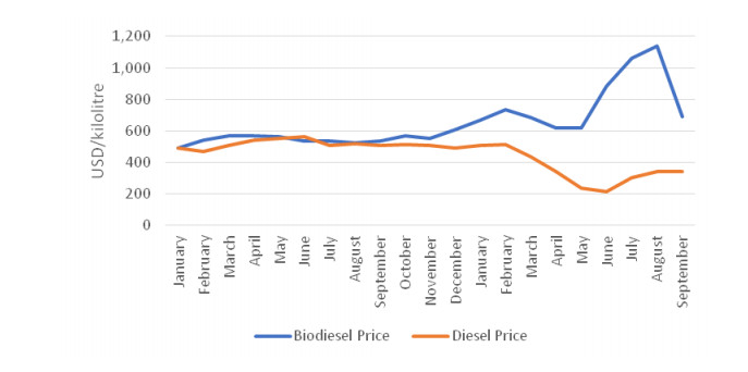
    [25] MEMR (2020) Market index price of biodiesel. Available from: http://ebtke.esdm.go.id/category/22/hip.bbn.
    [26] MIGAS B (2020) Market index price for subsidized and non subsidized gas oil to calculate the difference between market index price of gas oil with market index price of biodiesel. Available from: https://migas.esdm.go.id/uploads/harga-indek-pasar-/sept-2020---hip-minyak-solar--website-migas.pdf.
    [27] MoF (2015) Regulation of the minister of finance of the republic Indonesia no. 133/PMK.05/2015 In: Finance Mo, editor. Jakarta.
    [28] MoF (2018) Regulation of the minister of finance of the republic Indonesia no. 81/PMK.05/2018 Jakarta: Ministry of finance.
    [29] MoF (2019) Regulation of the minister of finance of the republic Indonesia no. 136/PMK.05/2019.
    [30] MoA (2020) Tree crop estate statistics of Indonesia 2018-2020: Palm oil. Jakarta: Directorate general of estates ministry of agriculture.
    [31] Nurfatriani F, Sari GK, Komarudin H (2019) Optimization of crude palm oil fund to support smallholder oil palm replanting in reducing deforestation in Indonesia. Sustainability 11: 4914.
    [32] Sterman J (2010) Business dynamics: Irwin/McGraw-Hill c2000.
    [33] Bautista S, Espinoza A, Narvaez P, et al. (2019) A system dynamics approach for sustainability assessment of biodiesel production in Colombia. Baseline simulation. J Cleaner Prod 213: 1-20.
    [34] MEMR (2019) FAQ: Program mandatori biodiesel 30% (B30). Directorate of new renewable energy and energy conservation, ministry of energy and mineral resources republic of Indonesia.
    [35] MoA (2018) Tree crop estate statistics of Indonesia 2017-2019 palm oil. Jakarta: Directorate general of estate crops, ministry of agriculture.
    [36] DGoP (2017) Guidelines for private oil plantations of planters, development of human resources and facilities and infrastructure assistance in the funding of the palm oil plantation fund management agency.
    [37] Asianagri (2019) Land rejuvenation success, oil palm farmers duplicate harvest production. Available from: https://www.asianagri.com/id/media-id/artikel/sukses-peremajaan-lahan-petani-kelapa-sawit-gandakan-hasil-panen.
    [38] MEMR (2015) Regulation of the minister of energy and mineral resources Indonesia about certain sector industry mandatory to use biodiesel and bioethanol as a fuel mixture with certain mixtures from 2015 to 2025. Minister of energy and mineral resources.
    [39] Indonesia PotRo (2014) Regulation of the president of the republic of Indonesia number 191 of 2014 concerning provision, distribution and retail price of oil fuel. Jakarta: President of Indonesia.
    [40] USDA (2019) Indonesia biofuels report 2019. Jakarta.
    [41] Migas B (2020) Konsumsi BBM nasional 2006-2018. Available from: https://www.bphmigas.go.id/kuota-dan-realisasi-jenis-bbm-tertentu/.
    [42] Population growth (annual %)-Indonesia, 2020. The World Bank Data.
    [43] BPDPKS (2019) PDPKS signs biodiesel incentive financing agreement for 2019. Palm oil fund management agency.
    [44] Barlas Y (1996) Formal aspects of model validity and validation in system dynamics. Syst Dyn Rev: J Syst Dyn Soc 12: 183-210.
    [45] Lawrence KD, Klimberg RK, Lawrence SM (2009) Fundamentals of forecasting using excel, Industrial Press Inc.
    [46] Arifin R (2019) RI wants to reach B50, car manufacturers say. Available from: https://oto.detik.com/mobil/d-4667356/ri-mau-loncat-ke-b50-ini-kata-produsen-mobil.
    [47] Sharon H, Karuppasamy K, Soban Kumar DR, et al. (2012) A test on DI diesel engine fueled with methyl esters of used palm oil. Renewable Energy 47: 160-166.
    [48] MEMR (2019) B30 road test results: All aspects of the vehicle have passed. Ministry of energy and mineral resources of the republic of Indonesia.
    [49] Sindo (2018) CPO export levy deleted, here are the facts (pungutan ekspor CPO dihapus, ini fakta-faktanya). Available from: https://economy.okezone.com/read/2018/11/27/320/1983508/pungutan-ekspor-cpo-dihapus-ini-fakta-faktanya.
    [50] Ogunkunle O, Ahmed NA (2019) A review of global current scenario of biodiesel adoption and combustion in vehicular diesel engines. Energy Reports 5: 1560-1579.
    [51] Gumilar P (2019) Gapki targets CPO productivity to be 6.9 tons per hectare per year. Available from: https://ekonomi.bisnis.com/read/20190412/99/910998/gapki-targetkan-produktivitas-cpo-jadi-69-ton-per-hektare-per-tahun.
    [52] Harahap F, Silveira S, Khatiwada D (2019) Cost competitiveness of palm oil biodiesel production in Indonesia. Energy 170: 62-72.
    [53] Amelia AR (2018) The government agrees to increase solar subsidies to rp 2,000 per liter, Available from: https://katadata.co.id/arnold/berita/5e9a55f50e96b/pemerintah-sepakat-naikkan-subsidi-solar-menjadi-rp-2000-per-liter.
    [54] Arvirianty A (2019) Biodiesel B30 is implemented in 2020, how much foreign exchange will be saved?: CNBC Indonesia. Available from: https://www.cnbcindonesia.com/news/20190619092850-4-79226/biodiesel-30-berlaku-2020-berapa-devisa-yang-dihemat.
    [55] Replanting is the key to improve livelihood of oil palm smallholders. 2018. Available from: https://www.bpdp.or.id/en/replanting-is-the-key-to-improve-oil-palm-smallholders-welfare.
    [56] Khatiwada D, Palmén C, Silveira SJB (2018) Evaluating the palm oil demand in Indonesia: production trends, yields, and emerging issues. Biofuels 1-13.
    [57] Population total-Indonesia, 2020. The World Bank Data.
    [58] Nurfatriani F, Sari GK, Komarudin H (2018) Optimalisasi dana sawit dan pengaturan instrumen fiskal penggunaan lahan hutan untuk perkebunan dalam upaya mengurangi deforestasi: CIFOR.
    [59] MIGAS B (2020) Laporan kinerja BPH migas tahun, 2019. BPH MIGAS.
  • Reader Comments
  • © 2020 the Author(s), licensee AIMS Press. This is an open access article distributed under the terms of the Creative Commons Attribution License (http://creativecommons.org/licenses/by/4.0)
通讯作者: 陈斌, bchen63@163.com
  • 1. 

    沈阳化工大学材料科学与工程学院 沈阳 110142

  1. 本站搜索
  2. 百度学术搜索
  3. 万方数据库搜索
  4. CNKI搜索

Metrics

Article views(8338) PDF downloads(497) Cited by(4)

Figures and Tables

Figures(9)  /  Tables(6)

/

DownLoad:  Full-Size Img  PowerPoint
Return
Return

Catalog