Figure 1.
The structure of the fault diagnosis method.


Citation: Rachael C. Adams, Behnam Rashidieh. Can computers conceive the complexity of cancer to cure it? Using artificial intelligence technology in cancer modelling and drug discovery[J]. Mathematical Biosciences and Engineering, 2020, 17(6): 6515-6530. doi: 10.3934/mbe.2020340
| [1] | Hamid Rastegari Kopaei, Mehdi Nooripoor, Ayatollah Karami, Myriam Ertz . Modeling consumer home composting intentions for sustainable municipal organic waste management in Iran. AIMS Environmental Science, 2021, 8(1): 1-17. doi: 10.3934/environsci.2021001 |
| [2] | Roberto Cavallo, Emanuela Rosio, Jacopo Fresta, Giada Fenocchio . Home composting in remote and cross-border areas of the In.Te.Se. project. AIMS Environmental Science, 2021, 8(1): 36-46. doi: 10.3934/environsci.2021003 |
| [3] | Carlos Garcia, Teresa Hernandez, Maria D Coll, Sara Ondoño . Organic amendments for soil restoration in arid and semiarid areas: a review. AIMS Environmental Science, 2017, 4(5): 640-676. doi: 10.3934/environsci.2017.5.640 |
| [4] | Lesly Mayive Latorre Malaver, Mauricio Cote-Alarcon . Sustainable use of paper sludge from the Colombian paper industry. AIMS Environmental Science, 2020, 7(3): 268-285. doi: 10.3934/environsci.2020017 |
| [5] | Katharina Meixner, Mona Kubiczek, Ines Fritz . Microplastic in soil–current status in Europe with special focus on method tests with Austrian samples. AIMS Environmental Science, 2020, 7(2): 174-191. doi: 10.3934/environsci.2020011 |
| [6] | Dongyan Mu, John Hawks, Andrew Diaz . Impacts on vegetable yields, nutrient contents and soil fertility in a community garden with different compost amendments. AIMS Environmental Science, 2020, 7(4): 350-365. doi: 10.3934/environsci.2020023 |
| [7] | Jerry R. Miller, John P. Gannon, Kyle Corcoran . Concentrations, mobility, and potential ecological risks of selected metals within compost amended, reclaimed coal mine soils, tropical South Sumatra, Indonesia. AIMS Environmental Science, 2019, 6(4): 298-325. doi: 10.3934/environsci.2019.4.298 |
| [8] | Serpil Guran . Options to feed plastic waste back into the manufacturing industry to achieve a circular carbon economy. AIMS Environmental Science, 2019, 6(5): 341-355. doi: 10.3934/environsci.2019.5.341 |
| [9] | Joseph Muiruri, Raphael Wahome, Kiemo Karatu . Assessment of methods practiced in the disposal of solid waste in Eastleigh Nairobi County, Kenya. AIMS Environmental Science, 2020, 7(5): 434-448. doi: 10.3934/environsci.2020028 |
| [10] | George Sikun Xu, Nicholas Chan . Management of radioactive waste from application of radioactive materials and small reactors in non-nuclear industries in Canada and the implications for their new application in the future. AIMS Environmental Science, 2021, 8(6): 619-640. doi: 10.3934/environsci.2021039 |
To ensure the safety and stable operation of industrial production within the industrial field, equipment fault diagnosis is extremely important. Because of the challenging atmosphere and harsh working circumstances, rolling bearings within mechanical equipment are often damaged [1]. According to statistics, rolling bearings are responsible for around 30% of mechanical faults in rotating equipment and about 20% of mechanical faults in gearboxes [2]. The rolling bearings' condition monitoring and fault diagnosis technology serve as an important tool in understanding the performance status of bearings and identifying potential faults in time [3]; in addition, it can effectively improve the operation management and maintenance efficiency of mechanical equipment, thus significantly improving the economic performance of enterprises [4].
Nowadays, gathering temperature or pressure data of the equipment for fault diagnosis does not yield accurate findings due to the influence of the factory's actual production process; alternatively, the equipment is directly connected to the vibration signal, which can therefore represent the device's operational status [5]. Thus, there is a high importance placed on research into fault diagnosis algorithms for vibration signals. In recent years, there has been a significant increase in computer performance due to advances in science and technology. Additionally, experts and academics have used machine learning and deep learning algorithms to diagnose faults using vibration signals [6]. Common fault diagnosis algorithms include support vector machine [7], k-nearest neighbor [8], random forest [9], convolution neural network (CNN) [10], long short-term memory (LSTM)[11] and transfer learning(TL) [12]. Wu [13] used the enhanced quantum-inspired differential evolution (MSIQDE) method to optimize deep confidence networks and facilitate fault diagnosis. Yuan [14] effectively utilized hypergraph algorithms to reduce the dimensionality of fault data features and implemented KNN classifiers for precise fault classification. Qing [15] proposed a novel Physical Information Residual Network (PIResNet) for the fault diagnosis of rolling bearings. Feng [16] created a digital replica of the gearbox's structure and employed a transfer learning algorithm to acquire knowledge on faults, which was then used to evaluate surface faults in an actual gearbox. Yuan [17] used the local-global standard hypergraph embedding (LGSHE) method to reduce the dimensionality of fault information and improve the accuracy of fault classification. Among them, CNN has attracted much attention because of its powerful feature extraction ability. Wang [18] employed a wavelet analysis to transform time-frequency picture data from one-dimensional (1D) vibration data into feature extraction and defect classification using a deep convolution neural network. Qiu [19] built a fault diagnosis model based on the CNN model by integrating auxiliary classifier generative adversarial network (ACGAN) and a self-attention mechanism. Gao [20] proposed a fault diagnosis method by combining maximum correlated kurtosis deconvolution (MCKD) and CNN. Hoang [21] transformed the 1D vibration signal into a binary graph and used CNN for fault diagnosis; however, this method lost the time series information. Wang [22] used improved Markov transformation field (MTF) to convert 1D vibration data into two-dimensional (2D) image data, and then used CNN to diagnose faults of rolling bearings. To achieve fault diagnosis, Zhao [23] proposed a new dimensionality reduction method and applied it to 1D-CNN with an adaptive activation function.
However, in the actual use of CNN for fault diagnosis, hyperparameters are often selected based on experience, which cannot allow CNN to play an optimal role, as the hyperparameter optimization problem for CNN has multi-modal characteristics [24]. Therefore, many scholars use intelligent optimization algorithms to optimize the hyperparameters of CNN. Sun [25] took the diagnosis accuracy and stability of the model as the optimization objective and used Differential Evolution (DE) to optimize the hyperparameters of CNN; however, the convergence speed was not satisfactory. Li [26] proposed a fault diagnosis method by combining the symplectic frog leapfrog algorithm (SFLA) and CNN, the SFLA is used to optimize the network structure and improve the feature extraction ability of CNN, thus improving the fault diagnosis accuracy of the model. Wang [27] combined auxiliary classifier generative adversarial network (VMD) with CNN for fault diagnosis by first optimizing the parameters of VMD and processing the data by using the improved grey wolf optimization algorithm; then, the processed data was inputted into the CNN, which optimized the model parameters through a grid search for fault diagnosis. However, the global search capability was not satisfactory.
Although CNN is an effective method in the field of rolling bearing fault diagnosis, there are still some challenges in practical applications such as quickly finding the most suitable hyperparameters and improving the feature representation ability of CNN models. To this end, this paper compares other intelligent optimization algorithms, and finds that though the DE algorithm has excellent global optimization ability [28], the iterative process of the grey wolf optimization (GWO) algorithm is quicker [29]. Therefore, this paper proposes a fault diagnosis algorithm that combines the two optimization algorithms to optimize the hyperparameters of the 1D convolutional neural network (1D-CNN) model and adds an attention mechanism after the 1D-CNN to highlight more useful fault feature information. Then, the algorithm uses the optimized 1D-CNN to build a fault diagnosis model to diagnose rolling bearing faults. The contribution of this paper can be summarized as follows:
1. A novel deep learning method based on 1D-CNN is proposed, which effectively enhances the fault feature information by adding an attention mechanism layer, prevents overfitting of the network by adding a dropout layer, and efficiently improves the accuracy of the classification.
2. A new swarm intelligence optimization algorithm based on DE-GWO is proposed, which not only enhances the global search ability, but also improves the convergence speed.
3. A fault diagnosis method for rolling bears based on DE-GWO-CNN is proposed, which efficiently identifies the best combination of six important hyperparameters for the improved 1D-CNN algorithm and effectively improves the fault diagnosis accuracy while ensuring fast convergence.
The remaining of this paper is displayed as follows. Section 2 represents the method used in this paper. Section 3 shows the training and testing datasets. The results and comparison are shown in Section 4 and the conclusion is drawn in Section 5.
The structure of the fault diagnosis method proposed in this paper is shown in Figure 1.
As seen from Figure 1, the first step is constructing the datasets involves normalizing fault signals and tags and dividing them into a training set and a test set. Next, we utilize the DE-GWO algorithm proposed in this paper to optimize the hyperparameters of the CNN method. Subsequently, we train the fault detection model using both the optimized CNN and the training data. Finally, we evaluate the trained model using a test set to ensure its accuracy and effectiveness.
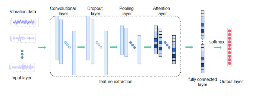
The main components of a 1D-CNN, which consists of a convolution layer, a pooling layer, and a fully connected layer, are similar to those of a typical feed-forward neural network. However, 1D-CNN has the added benefits of reducing model complexity, avoiding difficult feature extraction procedures, and reducing the number of weights required. The convolution, dropout, and pooling layers are utilized for feature extraction from the original signal, while the full connection layer creates a mapping relationship between the retrieved features and labels to realize the classification function. The structure of the 1D-CNN can be visualized in Figure 2.

The convolution layer applies a convolution operation to the input's original 1D data using convolution kernels, and then uses the activation function to make nonlinear changes to obtain a series of feature maps. The following formula [30] can be used to describe the convolution process:
| yi,j,k=f(s∑i=lxi,k∗wj,i+bi), | (1) |
where yi,j,k is the result of the convolution operation, f represents the activation function, which is Relu in this paper, xi,k represents the input data, * represents the convolution operation, wj,i represents weights and bi represents bias.
The dropout is used to prevent an overfitting problem during the training of the CNN model, which utilizes random sampling of weights based on a certain probability.
The purpose of the pooling operation is to improve the training speed of the convolution neural network and further avoid overfitting by reducing the dimension of the data. Popular pooling techniques include the maximum and average pooling methods; this paper adopts the maximum pooling method [30]:
| X=max(i−1)l+1⩽t⩽ilXl−1(t), | (2) |
where X represents the feature map after dimension reduction and l represents the length of the pooling area.
Finally, the extracted features are inputted into the full connection layer, the output probability is identified through the softmax function; then, the classification results are obtained. In this paper, before the full connection layer, a dropout layer is inserted to disregard some neurons and prevent overfitting during the training model.
Although 1D-CNN has a strong feature extraction ability, the selection of hyperparameters in the training process of the model will also have a great impact on the training results. At present, hyperparameters are generally selected through experience, though the effect is often general. This paper optimizes the hyperparameters of 1D-CNN by using the proposed DE-GWO algorithm.
The hyperparameters that have a great impact on the training results of 1D-CNN are the number of convolution kernels, the size of the convolution kernel, the dropout rate, the size of the pooling layer, the batch size and the learning rate. As a result, this paper mainly uses DE-GWO to optimize these parameters.
The attention mechanism can highlight the fault features with important information and suppress invalid features through adaptive weighting of different signal segments. The attention mechanism in this paper is added between the pooling layer and the fully connected layer. According to the attention mechanism, features that have a significant impact on the results will be given a greater weight. The structure is shown in Figure 3.

The input features are automatically extracted through convolution. The attention weight of each channel of the feature is obtained by adding an attention layer after the feature map. Then, the output feature map is produced using the dot product of the acquired attention weight and the original feature. The attention mechanism can be described as follows [31]:
| H′=MC(H)⊗H, | (3) |
where H∈n×m is the original feature map after the convolution operation, MC∈1×n is the attention weights for the channel dimensions, H′ is the feature map after the attention mechanism, ⊗ is the dot product, and MC(H) is described as follows [31]:
| MC(H)=σ(Conv([HCavg;HCmax])), | (4) |
where HCavg and HCmax are the global average pooling and global max pooling, respectively, Conv() is the convolution operation and σ is the activation function.
In this paper, the attention mechanism is added after the maxpooling layer to enhance the fault feature information of 1D-CNN.
In 1995, R. Storn and K. Price proposed the DE algorithm as a population-based optimization method. Compared with other optimization algorithms, the advantages of DE mainly lie in its controllability and few control parameters to be adjusted. Its attributes include a straightforward structure, straightforward realization, quick convergence, and high resilience; however, the convergence speed becomes slower during the latter part of the algorithm and sometimes even falls into the local best. In 2014, Mirjalili proposed the GWO algorithm as a population-based optimization method. It benefits from having a strong convergence performance, a straightforward structure, few adjustable parameters, and ease of implementation. When solving problems, it performs well in terms of convergence speed and accuracy. However, when faced with difficult issues, it easily converges early, and the convergence accuracy is not good. Narayan Nahak and Ranjan Kumar Mallick [32] combined the two algorithms into one by considering the final population of DE as the initial population of GWO, which took the advantages of both DE and GWO.
The traditional DE algorithm has a strong global search ability, though its convergence rate is not satisfactory. This paper effectively improves the rate of convergence and accuracy of the algorithm by integrating the GWO algorithm into the mutation process of DE, which makes the population evolution more directional. Figure 4 depicts the method's organizational structure.

The DE-GWO algorithm's operational approaches are as follows.
Step 1. Population initialization
The standard DE algorithm uses real number coding. First, generate an initial population with a scale of [N, D]. N represents the number of individuals in the population, and D represents the number of decision variables. The initial population can be expressed as follows:
| x={x1,D,x2,D,⋯,xN,D}, | (5) |
where x represents the initial population and xi,D represents an individual in the population.
Step 2. Mutation operation with GWO
The mutation operator used by the traditional mutation strategy is shown as follows [33]:
| Vi,g=Xr0,g+F(Xr1,g−Xr2,g),i≠r0≠r1≠r2, | (6) |
where Vi,g is a mutation individual, Xr0,g, Xr1,g and Xr2,g are individuals randomly selected from the population which are different from each other, and F is the scaling factor, which is usually a float data type set between 0 and 2.
However, in this paper, the mutation operation is completed by GWO. The following are the precise steps of the operation. First, make a fitness calculation for each person in the population. The individuals of the first three optimal solutions are called the head wolf, represented by α, β and δ, respectively, and the other individuals are grey wolves. Grey wolves update their hunting positions by simulating the hunting process according to the positions of the three head wolves. The mathematical formula for this process of hunting is as follows [34]:
| Dα=|C1Xα(t)−X(t)|, | (7) |
| Dβ=|C2Xβ(t)−X(t)|, | (8) |
| Dδ=|C3Xδ(t)−X(t)|, | (9) |
| X1=Xα(t)−A1Dα, | (10) |
| X2=Xβ(t)−A2Dβ, | (11) |
| X3=Xδ(t)−A3Dδ, | (12) |
where X represents an individual in the population, C represents the wobble factor, which is usually a float data type set randomly between 0 and 2, D represents the distance between the head wolves and the grey wolves, and A represents the convergence factor, which can decide whether the grey wolves move towards the head wolves' position. The new position of the individual in the population is expressed as follows:
| X(t+1)=X1+X2+X33, | (13) |
where X(t+1) represents an individual in the next generation population.
Finally, after all grey wolves have updated their positions, the new population is the mutation population of the DE algorithm.
Step 3. Crossover operation
The population variety may be further increased using the crossover approach. In this paper, the binomial crossover is the employed crossover technique [33]:
| Uj,i,g={Vj,i,g,Xj,i,g,randj(0,1)⩽Crorj=jrandothers, | (14) |
where Uj,i,g represents a crossover individual and Cr is the crossover operator, which is often a float data type set at random between 0 and 1. The crossover individual is the mutation individual if randj(0,1)⩽Crorj=jrand, and the original individual for the others.
Step 4. Select operation
The selection strategy is the last step of the DE algorithm. The experimental vector obtained through the crossover and the mutation is compared with the original vector. In this paper, to solve the minimum optimization problem and to enter the next generation, individuals with smaller fitness functions are chosen. It can be stated as follows [33]:
| Xi,g+1={Ui,g,f(Ui,g)⩽f(Xi,g)Xi,g,others, | (15) |
where Xi,g+1 is the next generation, Ui,g is the individual after the crossover operation, Xi,g is the parent individual before the mutation and crossover operations, and f stands for the fitness function.
The Rolling Bearing Data Center at CWRU provided the defect diagnosis datasets for this study. This paper employs a 48k drive end bearing fault data, a 3 hp motor load, and a 1,730 rpm motor speed. Table 1 displays a description of the data.
| Fault Type | Fault Size | Fault Position | Training Data sets | Testing Data sets | Label |
| Inner Race Fault | 0.1778 | — | 320 | 80 | 0 |
| Ball Fault | 0.1778 | — | 320 | 80 | 1 |
| Outer Race Fault | 0.1778 | Centered@6:00 | 320 | 80 | 2 |
| Inner Race Fault | 0.3556 | — | 320 | 80 | 3 |
| Ball Fault | 0.3556 | — | 320 | 80 | 4 |
| Outer Race Fault | 0.3556 | Centered@6:00 | 320 | 80 | 5 |
| Inner Race Fault | 0.5334 | — | 320 | 80 | 6 |
| Ball Fault | 0.5334 | — | 320 | 80 | 7 |
| Outer Race Fault | 0.5334 | Centered@6:00 | 320 | 80 | 8 |
| Normal | — | — | 320 | 80 | 9 |
 DownLoad:
CSV
DownLoad:
CSV
The experimental data consist of 10 types, including 9 fault types and 1 normal type. At the hour mark, the inner race, ball, and outside race are where the fault is placed; the corresponding fault diameters are 0.1778 mm, 0.3556 mm, and 0.5334 mm, respectively. Each type has 400 samples, of which 320 serve as training data sets and 80 serve as test data sets; each sample includes 1024 vibration data. To solve the problem that classifiers are not good at processing attribute data, the one-hot coding is used to replace the real number encoding.
The JNU datasets, obtained from Jiangnan University in China [35], is a comprehensive collection of bearing data. The datasets were generated using a centrifugal fan system test bed specifically designed for fault diagnosis. The test bed utilized a Mitsubishi SB-JR induction motor, with the rotor supported by two bearings, one of which was intentionally faulty. To capture the vibration signals, accelerometers were strategically placed in the vertical direction of the bearings. The datasets consider four distinct health states: normal condition (N), inner ring failure (IF), outer ring failure (OF), and rolling body failure (BF). The vibration acceleration signals were meticulously collected at three different speeds - 600,800, and 1000 rpm - with a sampling frequency of 50 kHz, ensuring rich and diverse datasets for various analytical purposes. In this paper, four operating states of the tachometer 600 are used to carry out troubleshooting experiments. Table 2 displays a description of the data.
| Fault Type | Training Data sets | Testing Data sets | Label |
| Inner Ring Failure (IF) | 400 | 80 | 0 |
| Outer Ring Failure (OF) | 400 | 80 | 1 |
| Rolling Body Failure (BF) | 400 | 80 | 2 |
| Normal | 400 | 80 | 3 |
DownLoad:
CSV
The experimental data in this study is comprised of four distinct types, with three fault types and one normal type. The faults are deliberately placed in the inner ring, outer ring, and rolling body of the bearing. For each type, there are 480 available samples, with 400 samples designated as training data sets and 80 samples as test data sets. Each sample contains 1,024 data points of vibration information, thereby providing ample data for analysis and model training.
This article opted not to process the data, and instead conducted an analysis and research using the original datasets. The objective was to preserve the salient features of the original signal with the utmost fidelity, thus enabling a better comprehension of the intrinsic properties and characteristics of the data.
The test was conducted on a computer with an i7-12700 CPU, featuring a main frequency of 3.6 GHz and 32 GB of memory. The programming software used was Python 3.9.7, with the TensorFlow2.0 environment developed by Google. The framework utilized was Keras, and the model was sequential.
To verify the optimization ability of the proposed algorithm under unimodal and multimodal functions, four standard test functions [36][37] are selected and used for simulation experiments, where the functions F1–F2 are unimodal, whereas F3–F4 are multimodal, and the proposed algorithm's convergence results are contrasted with those of other optimization algorithms and the optimization performance is analyzed. The expressions, search intervals and theoretical optimal values of the four standard test functions are listed in Table 3.
| Function | Function Expression | d | S | fmin |
| F1 | F1=d∑i=1x2i | 30 | [-100,100] | 0 |
| F2 | F2=d∑i=1|xi|+d∏i=1|xi| | 30 | [-10, 10] | 0 |
| F3 | F3=d∑i=1[x2i−10cos(2πxi)+10] | 30 | [-5.12, 5.12] | 0 |
| F4 | F4=−20exp(−0.2√1dd∑i=1x2i)−exp(1dd∑i=1cos2πxi)+20+e | 30 | [-32, 32] | 0 |
DownLoad:
CSV
To compare the proposed DE-GWO method, the DE method, and the GWO method's optimum performances, the three algorithms were used to solve the four standard test functions listed in Table 1. For the fairness of comparison, we set the population number to 30, the maximum number of iterations was 100, the crossover rates of DE-GWO and DE were both 0.5, and the mutation rate of DE was 0.5. For each test function, the three algorithms were independently run 20 times under the dimensions d = 30. The solution results are shown in Table 4.
| Test function | d | DE-GWO | DE | GWO | |||
| mean | SD | mean | SD | mean | SD | ||
| F1 | 30 | 2.42E-10 | 2.40E-10 | 1.27E+3 | 3.65E+2 | 1.82E-2 | 9.32E-2 |
| F2 | 30 | 2.95E-7 | 1.76E-7 | 1.77E+1 | 1.60E+0 | 2.49E-2 | 8.42E-3 |
| F3 | 30 | 3.24E-9 | 1.62E-9 | 2.12E+2 | 1.33E+1 | 3.18E+1 | 6.49E+0 |
| F4 | 30 | 4.31E-6 | 2.10E-6 | 8.94E+0 | 7.39E-1 | 2.3E-2 | 5.6E-3 |
DownLoad:
CSV
The table shows that the proposed DE-GWO algorithm performs better in terms of convergence accuracy and robustness compared to either the single DE or single GWO algorithms, whether in unimodal or multimodal functions. This supports the efficacy of the enhancement technique suggested in this research. Figure 5 displays the convergence curves of the methodologies for the four test functions.

The DE-GWO proposed in this paper is used to calculate the result in order to choose the hyperparameters of 1D-CNN with the highest fitness; then, the attention mechanism is added in the fault diagnosis model.
This paper chooses six hyperparameters that need to be optimized using DE-GWO in the 1D-CNN, as they have a great impact on the algorithm performance through numerous experiments, namely the number of convolution kernels, convolution step, dropout rate, pooling step, learning rate and batch size. An appropriate number of convolution kernels can avoid both underfitting and overfitting. The convolution step can affect the training speed and the ability of extract features. The dropout rate can effectively reduce the risk of overfitting of the model. The pooling step can control the complexity of the model. The learning rate can influence the convergence speed. The batch size has a significant impact on the convergence rate.
Before using the optimization algorithm, the value range of these six hyperparameters should be determined. According to experience, this paper sets the range of the number of convolution cores as 1 to 100, the convolution step size as 1 to 100, the dropout rate as 0.1 to 0.9, the pooling step size as 1 to 100, the batch size as 10 to 100, and the learning rate as 0 to 1.
The parameters of the DE-GWO algorithm are as follows: the maximum evolution times is 10, the number of populations is 10, the dimension is 6 and the cross probability is 0.5.
This paper uses rolling bearing data to train the model; the fitness function of the DE-GWO algorithm is as follows:
| f(xi,g)=Axi,g, | (16) |
where xi,g represents the ith individual of the g generation and Axi,g represents the loss result of one iteration of the 1D-CNN. Figure 6 shows the convergence curves of the three optimized algorithms for 1D-CNN.

After the optimization of the DE-GWO, DE and GWO, the fitness hyperparameters of the 1D-CNN using different algorithms and normal 1D-CNN with hyperparameters selected by experience are shown in Table 5.
| Algorithm | KC | KL | PL | Dropout | Learning Rate | Batch Size |
| DE-GWO | 10 | 64 | 9 | 0.26524 | 0.00423 | 42 |
| DE | 17 | 54 | 18 | 0.38586 | 0.00402 | 17 |
| GWO | 42 | 40 | 36 | 0.26008 | 0.00516 | 33 |
| normal | 8 | 8 | 3 | 0.2 | 0.004 | 40 |
DownLoad:
CSV
The padding of the model is the "same", the activation of the convolution layer is relu and the classifier is softmax. To enhance fault feature information of 1D-CNN, the attention mechanism is added after the maxpooling layer.
Taking categorical_crossentropy as the loss function to update model parameters, 80% of the data set is used as the training data set of the algorithm and the remaining 20% as the test data set. Then, DE-GWO-CNN with attention mechanism, DE-CNN, GWO-CNN and 1D-CNN are used to diagnose rolling bearing faults. The iteration number of the algorithm is set as 60. The fault diagnosis accuracy and loss function of the four algorithms are shown in Figure 7.

The four methods in the training set can all achieve 100% accuracy after 40 iterations; however, the approach suggested in this study has the fastest convergence speed, a smoother curve, and superior stability. Table 6 displays the various algorithms' fault diagnostic accuracy and validation time for the test data set. Though not statistically different from other algorithms, the proposed fault diagnosis method does not have the shortest validation time. However, its accuracy is the highest among these algorithms, indicating that it is effective for diagnosing faults in rolling bearings.
| Algorithm | KC | KL | PL | Dropout | Learning Rate | Batch Size |
| DE-GWO | 14 | 90 | 19 | 0.16168 | 0.00659 | 32 |
| GWO | 8 | 72 | 40 | 0.38763 | 0.00727 | 25 |
| DE | 58 | 50 | 22 | 0.38547 | 0.00519 | 12 |
| normal | 8 | 8 | 3 | 0.2 | 0.004 | 40 |
DownLoad:
CSV
To further clarify the diagnostic superiority of the algorithm proposed in this paper, the confusion matrix of the normal 1D-CNN, the improved 1D-CNN and the DE-GWO-CNN are compared with each other. The results are shown in Figure 8, which express the accuracy of different fault diagnosis benchmarks for different fault types.

The figure indicates that the proposed algorithm achieves a diagnostic accuracy of 100% for states one, five, seven, nine and ten, while the lowest diagnostic accuracy for the remaining five states is 97.5%. Compared to the normal 1D-CNN and the improved 1D-CNN, the proposed method achieves the highest accuracy, indicating that the fault diagnosis model presented in this paper has a superior diagnostic ability.
Taking categorical_crossentropy as the loss function to update model parameters, 75% of the data set is used as the training data set of the algorithm and the remaining 25% as the test data set. Then, DE-GWO-CNN with attention mechanism, DE-CNN, GWO-CNN and 1D-CNN are used to diagnose rolling bearing faults. The iteration number of the algorithm is set as 60. The fault diagnosis accuracy and loss function of the four algorithms are shown in Figure 9.

The GWO-CNN and DE-GWO-CNN algorithms achieved 100% accuracy after just 30 iterations in the training set, outperforming other methods that required more iterations. The proposed approach in this study exhibits the fastest convergence speed, a smoother curve, and superior stability. Table 7 presents the fault diagnostic accuracy and validation time for various algorithms on the test datasets. While the proposed fault diagnosis method does not have the shortest validation time, the difference is not significant compared to other algorithms. More importantly, the method achieves the highest accuracy among these algorithms, demonstrating its effectiveness in diagnosing faults in rolling bearings. This superior accuracy justifies the use of the proposed method for fault diagnosis in rolling bearing.
| Fault diagnosis model | DE-GWO-CNN | DE-CNN | GWO-CNN | 1D-CNN |
| Accuracy | 99.25% | 97.25% | 92.875% | 85.75% |
| Recall | 99.253% | 96.966% | 93.011% | 85.623% |
| F1 | 99.251% | 97.108% | 92.893% | 85.686% |
| Validation time (s/epoch) | 0.36 | 0.68 | 0.29 | 0.27 |
DownLoad:
CSV
To further demonstrate the diagnostic superiority of the algorithm proposed in this paper, a comparison of confusion matrices is conducted between the normal 1D-CNN, the DE-CNN, the GWO-CNN and the DE-GWO-CNN. As shown in Figure 10, the results illustrate the accuracy of different fault diagnosis methods for various fault types. This comparison effectively highlights the improved performance of the proposed algorithm.

Using Figure 10, the average recognition accuracy for each operating condition of different algorithms is calculated and the results are listed in Table 8.
| Fault diagnosis model | DE-GWO-CNN | GWO-CNN | DE-CNN | 1D-CNN |
| Accuracy | 99.69% | 95.00% | 92.43% | 83.13% |
| Precision | 99.69% | 95.00% | 92.43% | 83.13% |
| Recall | 100% | 95.02% | 93.68% | 84.22% |
| F1 | 99.84% | 95.01% | 93.05% | 83.67% |
| Validation time (s/epoch) | 0.36 | 0.46 | 0.28 | 0.22 |
DownLoad:
CSV
According to the table, the proposed algorithm demonstrates a diagnostic accuracy of 100% for states one, three, and four, with a slightly lower accuracy of 98.75% for the remaining states. In comparison to other algorithms, the proposed method exhibits the highest accuracy. These results indicate that the fault diagnosis model presented in this paper possesses superior diagnostic capabilities.
To demonstrate the superiority of the proposed fault diagnosis algorithm, a quantitative comparison was made between the algorithm proposed in this paper and DE-GWO-CNN without an attention mechanism, as well as three classic models: GoogLeNet, LeNet-5, and AlexNet. All models were trained on the CWRU datasets but with different hyperparameters. The test results are presented in Table 9.
| Fault diagnosis model | DE-GWO-CNN | GWO-CNN | DE-CNN | 1D-CNN |
| IF | 100% | 95.00% | 91.25% | 88.75% |
| OF | 98.75% | 95.00% | 96.25% | 81.25% |
| BF | 100% | 92.50% | 87.50% | 65.00% |
| Normal | 100% | 97.50% | 98.75% | 97.50% |
DownLoad:
CSV
| Fault diagnosis model | Accuracy |
| The proposed method | 99.25% |
| DE-GWO-CNN without attention mechanism | 94.50% |
| GoogLeNet | 93.75% |
| LeNet-5 | 91.87% |
| AlexNet | 96.13% |
DownLoad:
CSV
According to the table, when compared to DE-GWO-CNN without attention mechanism, GoogLeNet, LeNet-5, and AlexNet, the proposed algorithm demonstrates a superior accuracy in fault diagnosis. Specifically, the proposed method achieves 4.75%, 5.5%, 7.48%, and 2.92% higher accuracy than these respective models. This suggests that the proposed algorithm may offer a more effective solution for fault diagnosis.
Finally, to verify the anti-noise ability of the algorithm proposed in this paper, Gaussian white noise is added to the original rolling bearing vibration data, and the signal-noise ratio (SNR) is used to measure the noise, which is shown as follows [38]:
| SNR=10log10PsignalPnoise | (17) |
where Psignal represents the power of the signal and Pnoise represents the power of the noise.
This paper sets up three sets of noise experiments, with signal-to-noise ratios of -5 dB, 5 dB, and 10 dB. The four algorithms used for fault diagnosis are DE-GWO-CNN, DE-CNN, GWO-CNN, and normal 1D-CNN. The results are presented in Figure 11.

The experimental findings clearly demonstrate that the suggested algorithm outperforms the other three algorithms in terms of fault diagnostic performance for these three types of Gaussian white noise. Moreover, the results also highlight the program's exceptional anti-noise capability and its potential for higher engineering application value.
While the 1D-CNN algorithm is effective in feature extraction, selecting optimal hyperparameters can be challenging and its feature representation ability may not always be satisfactory. To address these issues, we propose a novel approach that utilizes the DE-GWO intelligent optimization algorithm to optimize the hyperparameters of 1D-CNN. By finding the most suitable hyperparameters, our method enhances the ability of the 1D-CNN model to extract features from bearing vibration signals and improve the fault classification accuracy. Additionally, we enhance the feature representation ability of 1D-CNN by incorporating an attention mechanism. Comparative tests demonstrate that our proposed algorithm improves the accuracy and convergence speed of fault diagnosis. Notably, the algorithm exhibits high anti-noise performance, as it achieves a relatively higher accuracy even when the signal-to-noise ratio is set to -5 dB, 5 dB, and 10 dB.
Furthermore, although the diagnostic accuracy of the rolling bearing fault diagnosis model proposed in this paper is reasonably high, there is still room for improvement in terms of its transferability. Therefore, our future research efforts will be focused on enhancing the transferability of the fault diagnosis model, with the aim of facilitating its broader application in real-world industrial settings.
The authors declare they have not used Artificial Intelligence (AI) tools in the creation of this article.
This research was supported by Key Research and Development Project of Liaoning Province (Grant No. 2020JH2/10300040); Applied Basic Research Project of Liaoning Province, China (Grant No. 2023JH2/101300183).
All authors declare that no conflict of interest exists.
| [1] | R. Mahumad, K. Alam, J. Dunn, J. Gow, Emerging cancer incidence, mortality, hospitalisation and associated burden among Australian cancer patients, 1982-2014: An incidence-based approach in terms of trends, determinants and inequality, BMJ Open, 5 (2019). |
| [2] | M. Breitenbach, J. Hoffmann, Editorial: Cancer models, Front. Oncol., 8 (2018), 401-401. |
| [3] | L. Ogilvie, A. Kovachev, C. Wierling, B. Lange, H. Lehrach, Models of models: A translational Route for cancer treatment and drug development, Front. Oncol., 7 (2017). |
| [4] | K. Mak, M. Pichika, Artificial intelligence in drug development: Present status and future prospects, Drug Discovery Today, 24 (2019), 773-780. |
| [5] | J. Vamathevan, D. Clark, P. Czodrowski, I. Dunham, E. Ferran, G. Lee, et al., Applications of machine learning in drug discovery and development, Nat. Rev. Drug Discovery, 18 (2018), 463-477. |
| [6] | O. Wolkenhauer, Why model? Front. Phys., 5 (2014). |
| [7] | A. Levine, C. Schlosser, J. Grewal., R. Coope, S. Jones, S. Yip, Rise of the machines: Advances in deep learning for cancer diagnosis, Trends Cancer, 5 (2019), 157-169. |
| [8] | K. Vougas, T. Sakellaropolous, A. Kotsina, G. R. P. Foukas, A. Ntargaras, F. Koinis, et al., Machine learning and data mining frameworks for predicting drug response in cancer: An overview and a novel in silico screening process based on association rule mining. Pharmacol. Ther., 203 (2019), 107395. |
| [9] | G. V. Sherbet, W. L. Woo, S. Dlay, Application of artificial intelligence-based technology in cancer management: A commentary on the deployment of artificial neural networks, Anticancer Res., 38 (2018), 6607-6613. |
| [10] | R. M. Thomas, T. Van Dyke, G. Merlino, C. P. Day, Concepts in cancer modeling: A brief history, Cancer Res., 76 (2016), 5921-5925. |
| [11] | P. Kumari, A. Nath, R. Chaube, Identification of human drug targets using machine-learning algorithms, Comput. Biol. Med., 56 (2014), 175-181. |
| [12] | J. Metzcar, Y. Wang, R. Heiland, P. Macklin, A Review of cell-based computational modeling in cancer biology, JCO Clin. Cancer Inform., 3 (2019), 1-13. |
| [13] | D. Hanahan, R. A. Weinberg, The hallmarks of cancer, Cell, 100 (2000), 57-70. |
| [14] | A. Ghaffarizadeh, S. H. Friedman, P. Macklin, BioFVM: An efficient, parallelized diffusive transport solver for 3-D biological simulations, Bioinformatics, 32 (2016), 1256-1258. |
| [15] | A. Ghaffarizadeh, R. Heiland, S. H. Friedman, S. M. Mumethaler, P. Macklin, PhysiCell: An open source physics-based cell simulator for 3-D multicellular systems, PLOS Comput. Biol., 14 (2018), e1005991. |
| [16] | E. Bonabeau, Agent-based modeling: Methods and techniques for simulating human systems, Proc. Natl. Acad. Sci. USA, 99 (2002), 7280-7287. |
| [17] | P. Van Liedekerke, M. M. Palm, N. Jagiella, D. Drasdo, Simulating tissue mechanics with agent-based models: Concepts, perspectives and some novel results, Comput. Particle Mech., 2 (2015), 401-444. |
| [18] | R. C. Kennedy, G. E. Ropella, C. A. Hunt, A cell-centered, agent-based framework that enables flexible environment granularities, Theor. Biol. Med. Model. 13 (2016). |
| [19] | J. Poleszczuk, P. Macklin, H. Enderling, Agent-based modeling of cancer stem cell driven solid tumor growth, Methods Mol. Biol., 1516 (2016), 335-346. |
| [20] | Y. Cai, S. Xu, J. Wu, Q. Long, Coupled modelling of tumour angiogenesis, tumour growth and blood perfusion, J. Theor. Biol., 279 (2011), 90-101. |
| [21] | A. Shirinifard, J. S. Gens, B. L. Zaitlen, N. J. Poplawski, M. Swat, J. A. Glazier, 3D multi-cell simulation of tumor growth and angiogenesis, PLOS One, 4 (2009), e7190. |
| [22] | B. Chopard, R. Ouared, A. Deustch, H. Hatzikirou, D. Wolf-Gladrow, Lattice-gas cellular automaton models for biology: From fluids to cells, Acta Biotheor., 58 (2010), 329-340. |
| [23] | H. Hatzikirou, D. Basanta, M. Simon, K. Schaller, A. Deustch, 'Go or Grow': The key to the emergence of invasion in tumour progression?, Math. Med. Biol.: A J. IMA, 29 (2010), 49-65. |
| [24] | H. N. Weerasinghe, P. M. Burragem, K. Burrage, D. V. Nicolau, Mathematical models of cancer cell plasticity, J. Oncol., 2019. |
| [25] | M. S. Alber, M. A. Kiskowski, J. A. Glazier, Y. Jiang, On cellular automaton approaches to modeling biological cells, in Mathematical Systems Theory in Biology, Communications, Computation, and Finance, Springer, New York, (2003), 1-39. |
| [26] | A. Szabó, R. M. Merks, Cellular potts modeling of tumor growth, tumor invasion, and tumor evolution, Front. Oncol., 3 (2013). |
| [27] | N. Guisoni, K. I. Mazzitello, L. Diambra, Modeling active cell movement with the potts model, Front. Phys., 6 (2018). |
| [28] | E. G. Rens, L. Edelstein-Keshet, From energy to cellular forces in the cellular potts model: An algorithmic approach, PLOS Comput. Biol., 15 (2019), e1007459. |
| [29] | K. A. Rejniak, A. R. A. Anderson, Hybrid models of tumor growth, Wiley Interdiscip. Rev.: Syst. Biol. Med., 3 (2011), 115-125. |
| [30] | J. Jeon, V. Quaranta, P. T. Cummings, An off-lattice hybrid discrete-continuum model of tumor growth and invasion, Biophys. J., 98 (2010), 37-47. |
| [31] | S. Koride, A. J. Loza, S. X. Sun, Epithelial vertex models with active biochemical regulation of contractility can explain organized collective cell motility, APL Bioeng., 2 (2018). |
| [32] | S. Alt, P. Ganguly, G. Salbreux, Vertex models: from cell mechanics to tissue morphogenesis, Philos. Tran. R. Soc. London. Ser. B, Biol. Sci., 372 (2017). |
| [33] | K. R. Foster, R. Koprowski, J. D. Skufca, Machine learning, medical diagnosis, and biomedical engineering research-commentary, Biomed. Eng. Online, 13 (2014), 94. |
| [34] | A. M. Shirin, S. S. Dlay, W. L. Woo, G. V. Sherbet, Cross validation evaluation for breast cancer prediction using multilayer perceptron neural networks, Am. J. Eng. Appl. Sci., 4 (2012). |
| [35] | T. Dietterich, Overfitting and undercomputing in machine learning, ACM Comput. Surveys, 27 (1995), 326-327. |
| [36] | T. L. Whiteside, The tumor microenvironment and its role in promoting tumor growth, Oncogene, 27 (2018), 5904-5912. |
| [37] | D. Hanahan, R. A. Weinberg, Hallmarks of cancer: the next generation, Cell, 144 (2011), 646-674. |
| [38] | A. M. Newman, C. B. Steen, C. L. Liu, A. J. Gentles, A. A. Chaudhuri, F. Scherer, et al., Determining cell type abundance and expression from bulk tissues with digital cytometry. Nat. Biotech., 37 (2019), 773-782. |
| [39] | B. Chen, M. S. Khodadoust, C. L. Liu, A. M. Newman, A. A. Alizadeh, Profiling tumor infiltrating immune cells with CIBERSORT, Methods Mol. Biol., 1711 (2018), 243-259. |
| [40] | K. Menden, M. Marouf, S. Oller, A. Dalmia, D. S. Magruder, K. Kloiber, et al., Deep learning-based cell composition analysis from tissue expression profiles, Sci. Adv., 6 (20100), eaba2619. |
| [41] | X. Sun, B. Hu, Mathematical modeling and computational prediction of cancer drug resistance, Brief Bioinf., 19 (2018), 1382-1399. |
| [42] | J. Cosgrove, J. Butler, K. Alden, M. Read, V. Kumar, L. Cucurull-Sanchez, et al., Agent-based modeling in systems pharmacology, CPT: Pharmacometrics Syst. Pharmacol., 4 (2015), 615-629. |
| [43] | R. L. Dedrick, D. S. Zaharko, R. A. Bender, W. A. Bleyer, R. J. Lutz, Pharmacokinetic considerations on resistance to anticancer drugs, Cancer Chemother Rep., 59 (1975), 795-804. |
| [44] | H. B. Frieboes, M. E. Edgerton, J. P. Fruehauf, F. R. A. J. Rose, L. K. Worrall, R. A. Gatenby, et al., Prediction of drug response in breast cancer using integrative experimental/computational modeling, Cancer Res., 69 (2009, 4484-4492. |
| [45] | B. G. Birkhead, E. M. Rankin, S. Gallivan, L. Dones, R. D. Rubens, A mathematical model of the development of drug resistance to cancer chemotherapy, Eur. J. Cancer Clin. Oncol., 23 (1987), 1421-1427. |
| [46] | A. Ghaffarizadeh, S. H. Friedman, P. Macklin, BioFVM: an efficient, parallelized diffusive transport solver for 3-D biological simulations, Bioinformatics, 32 (2015), 1256-1258. |
| [47] | E. F. Juarez, R. Lau, S. H. Friedman, A. Ghaffarizadeh, E. Jonckheere, D. B. Agus, et al., Quantifying differences in cell line population dynamics using CellPD, BMC Syst. Biol., 10 (2016). |
| [48] | S. H. Friedman, A. R. A. Anderson, D. M. Bortz, A. G. Fletcher, H. B. Frieboes, A. Ghaffarizadeh, et al., MultiCellDS: a standard and a community for sharing multicellular data, preprint, bioRxiv 090696. |
| [49] | H. C. Tang, Y. C. Chen, Insight into molecular dynamics simulation of BRAF(V600E) and potent novel inhibitors for malignant melanoma, Int. J. Nanomedicine, 10 (2015), 3131-3146. |
| [50] | K. J. Mahasa, R. Ouifki, A. Eladdadi, L. de Pillis, Mathematical model of tumor-immune surveillance, J. Theor. Biol., 404 (2016), 312-330. |
| [51] | T. Jackson, A. Radunskaya, Applications of Dynamical Systems in Biology and Medicine, 2015. |
| [52] | A. Dhawan, T. A. Graham, A. G. Fletcher, A computational modeling approach for deriving biomarkers to predict cancer risk in premalignant disease, Cancer Prev. Res., 9 (2016), 283-295. |
| [53] | X. Yang, Y. Wang, R. Byrne, G. Schneider, S. Yang, Concepts of artificial intelligence for computer-assisted drug discovery, Chem. Rev., 119 (2019), 10520-10594. |
| [54] | W. Kolch, D. Fey, Personalized computational models as biomarkers, J. Pers. Med., 7 (2017), 9. |
| [55] | C. L. Fischer, A. M. Bates, E. A. Lanzel, J. M. Guthmiller, G. K. Johnson, N. K. Singh, et al., Computational models accurately predict multi-cell biomarker profiles in inflammation and cancer, Sci. Rep., 9 (2019), 10877. |
| [56] | F. J. Esteva, G. N. Hortobagyi, Prognostic molecular markers in early breast cancer, Breast Cancer Res., 6 (2004), 109-118. |
| [57] | S. Mojarad, B. Venturini, P. Fulgenzi, R. Papaleo, M. Brisigotti, F. Monti, et al., Prediction of nodal metastasis and prognosis of breast cancer by ANN-based assessment of tumour size and p53, Ki-67 and steroid receptor expression, Anticancer Res., 33 (2013), 3925-3933. |
| [58] | M. P. Menden, F. Iorio, M. Garnett, U. McDermott, C. H. Benes, P. J. Ballester, et al., Machine learning prediction of cancer cell sensitivity to drugs based on genomic and chemical properties, Plos One, 8 (2013), e61318. |
| [59] | A. Bravo, J. Pinero, N. Queralt-Rosinach, M. Rautschka, L. I. Furlong, Extraction of relations between genes and diseases from text and large-scale data analysis: implications for translational research, BMC Bioinfor., 16 (2015). |
| [60] | J. Kim, J-j. Kim, H. Lee, An analysis of disease-gene relationship from medline abstracts by DigSee, Sci. Rep., 7 (2017), 40154. |
| [61] | P. Mamoshina, M. Volosnikova, I. V. Ozerov, E. Putin, E. Skibina, F. Cortese, et al., Machine learning on human muscle transcriptomic data for biomarker discovery and tissue-specific drug target identification, Front. Genet., 9 (2018). |
| [62] | T. Zhu, S, Cao, P. C. Su, R. Patel, D. Shah, H. B. Chokshi, et al., Hit identification and optimization in virtual screening: Practical recommendations based on a critical literature analysis, J. Med. Chem., 56 (2013), 6560-6572. |
| [63] | G. Klopman, S. K. Chakravarti, H, Zhu, J. M. Ivanov, R. D. Saiakhov, ESP: A method to predict toxicity and pharmacological properties of chemicals using multiple MCASE databases, J. Chem. Infor. Comput. Sci., 44 (2004), 704-715. |
| [64] | I. W. Mak, N. Evaniew, M. Ghert, Lost in translation: animal models and clinical trials in cancer treatment, Am. J. Trans. Res., 6 (2014), 114-118. |
| [65] | B. Ramsundar, B. Liu, Z. Wu, A. Verra, M. Tudor, R. P. Sherridan, et al., Is multitask deep learning practical for pharma?, J. Chem. Infor. Model., 57 (2017), 2068-2076. |
| [66] | M. Olivecrona, T. Blashcke, O. Engvist, H. Chen, Molecular de-novo design through deep reinforcement learning, J. Cheminfor., 9 (2017). |
| [67] | T. Luechtefeld, D. Marsh, C. Rowlands, T. Hartung, Machine learning of toxicological big data enables read-across structure activity relationships (RASAR) outperforming animal test reproducibility, Toxicol. Sci., 165 (2018), 198-212. |
| [68] | J. L. Perez-Gracia, M. F. Sanmamed, A. Bosch, A. Patino-Garcia, K. A. Schalper, V. Segura, et al., Strategies to design clinical studies to identify predictive biomarkers in cancer research, Cancer Treat. Rev., 53 (2017), 79-97. |
| [69] | E. E. Bain, L. SHafner, D. P. Walling, A. A. Othman, C. C. Stein, J. Hinkle, et al., Use of a novel artificial intelligence platform on mobile devices to assess dosing compliance in a Phase 2 clinical trial in subjects with schizophrenia, JMIR mHealth uHealth, 5 (2017), e18. |
| [70] | A. H. Beck, A. R. Sangoi, S. Leung, R. K. Marinelli, T. O. Nielsen, M. J. van de Vijver, et al., Systematic analysis of breast cancer morphology uncovers stromal features associated with survival, Sci. Trans. Med., 3 (2011). |
| [71] | N. L. Mani, K. A. Schalper, C. Hatzis, O. Saglam, F. Tavassoli, M. Butler, et al., Quantitative assessment of the spatial heterogeneity of tumor-infiltrating lymphocytes in breast cancer, Breast Cancer Res., 18 (2016). |
| [72] | F. Lake, Artificial intelligence in drug discovery: what is new, and what is next?, Future Drug Discovery, 1 (2019). |
| [73] | K. L. Fetah, B. J. DiPArdo, E. M. Kongadzem, J. S. Tomlinson, A. Elzaghied, M. Elmusrati, et al., Cancer modeling-on-a-chip with future artificial intelligence integration, Small, 15 (2019). |
| [74] | V. Assadollahi, B. Rashidieh, M. Alasvand, A. Abdolahi, J. A. Lopez, Interaction and molecular dynamics simulation study of Osimertinib (AstraZeneca 9291) anticancer drug with the EGFR kinase domain in native protein and mutated L844V and C797S, J. Cell. Biochem., 120 (2019), 13046-13055. |
| [75] | S. Ghafari, M. Komeilian, M. Hashemi, S. Oushani, G. Rigi, B. Rashidieh, et al., Molecular docking based screening of Listeriolysin-O for improved inhibitors, Bioinformation, 13 (2017), 160-163. |
| [76] | V. Assadollahi, B. Rashidieh, Molecular dynamics simulation of EFGR L844V mutant sensitive to AZD9291 in non-small cell lung cancer, J. Thorac. Oncol., 12 (2017), 1210. |
| [77] | M. M. Ranbar, V. Assadolahi, M. Yazdani, D. Nikaein, B. Rashidieh, Virtual dual inhibition of COX-2/5-LOX enzymes based on binding properties of alpha-amyrins, the anti-inflammatory compound as a promising anti-cancer drug, EXCLI J., 15 (2016), 238-245. |
| [78] | B. Rashidieh, M. Valizadeh, V. Assadollahi, M. M. Ranjbar, Molecular dynamics simulation on the low sensitivity of mutants of NEDD-8 activating enzyme for MLN4924 inhibitor as a cancer drug, Am. J. Cancer Res., 5 (2015), 3400-3406. |
| [79] | B. Rashidieh, Z. Madani. M. K. Azam, S. K. Maklavani, N. R. Akbari, S. Tavakoli, et al., Molecular docking based virtual screening of compounds for inhibiting sortase A in L. monocytogenes, Bioinformation, 11 (2015), 501-505. |
| [80] | B. Rashidieh, S. Etemadiafshar, G. Memari, M. Mirzaeichegeni, S. Yazdi, F. Farsimadan, et al., A molecular modeling based screening for potential inhibitors to alpha hemolysin from Staphylococcus aureus, Bioinformation, 11 (2015), 373-377. |
| [81] | J. Ozik, N. Collier, R. Heiland, G. An, P. Macklin, Learning-accelerated discovery of immune-tumour interactions, Mol. Syst. Des. Eng., 4 (2019), 747-760. |
| [82] | J. Ozik, N. Collier, J. M. Wozniak, C. Macal, C. Cockrell, S. F. Friedman, et al., High-throughput cancer hypothesis testing with an integrated PhysiCell-EMEWS workflow, BMC Bioinfor., 19 (2018). |
| 1. | Atilla Kunszabó, Dávid Szakos, Annamária Dorkó, Csilla Farkas, Gyula Kasza, Household food waste composting habits and behaviours in Hungary: A segmentation study, 2022, 30, 23525541, 100839, 10.1016/j.scp.2022.100839 | |
| 2. | Haniyeh Jalalipour, Azadeh Binaee Haghighi, Navarro Ferronato, Sara Bottausci, Alessandra Bonoli, Michael Nelles, Social, economic and environmental benefits of organic waste home composting in Iran, 2024, 0734-242X, 10.1177/0734242X241227377 | |
| 3. | Ana Catarina Morais, Akira Ishida, Composting behavior in Japan: an application of the theory of consumption values, 2025, 8, 2571-581X, 10.3389/fsufs.2024.1435898 | |
| 4. | Ana Catarina Morais, Akira Ishida, Reasons to dropout household composting among Japanese, 2025, 1932-0248, 1, 10.1080/19320248.2025.2494045 |
Figures(1) / Tables(1)

Rachael C. Adams, Behnam Rashidieh. Can computers conceive the complexity of cancer to cure it? Using artificial intelligence technology in cancer modelling and drug discovery[J]. Mathematical Biosciences and Engineering, 2020, 17(6): 6515-6530. doi: 10.3934/mbe.2020340

| Fault Type | Fault Size | Fault Position | Training Data sets | Testing Data sets | Label |
| Inner Race Fault | 0.1778 | — | 320 | 80 | 0 |
| Ball Fault | 0.1778 | — | 320 | 80 | 1 |
| Outer Race Fault | 0.1778 | Centered@6:00 | 320 | 80 | 2 |
| Inner Race Fault | 0.3556 | — | 320 | 80 | 3 |
| Ball Fault | 0.3556 | — | 320 | 80 | 4 |
| Outer Race Fault | 0.3556 | Centered@6:00 | 320 | 80 | 5 |
| Inner Race Fault | 0.5334 | — | 320 | 80 | 6 |
| Ball Fault | 0.5334 | — | 320 | 80 | 7 |
| Outer Race Fault | 0.5334 | Centered@6:00 | 320 | 80 | 8 |
| Normal | — | — | 320 | 80 | 9 |
DownLoad:
CSV
| Fault Type | Training Data sets | Testing Data sets | Label |
| Inner Ring Failure (IF) | 400 | 80 | 0 |
| Outer Ring Failure (OF) | 400 | 80 | 1 |
| Rolling Body Failure (BF) | 400 | 80 | 2 |
| Normal | 400 | 80 | 3 |
DownLoad:
CSV
| Function | Function Expression | d | S | fmin |
| F1 | F1=d∑i=1x2i | 30 | [-100,100] | 0 |
| F2 | F2=d∑i=1|xi|+d∏i=1|xi| | 30 | [-10, 10] | 0 |
| F3 | F3=d∑i=1[x2i−10cos(2πxi)+10] | 30 | [-5.12, 5.12] | 0 |
| F4 | F4=−20exp(−0.2√1dd∑i=1x2i)−exp(1dd∑i=1cos2πxi)+20+e | 30 | [-32, 32] | 0 |
DownLoad:
CSV
| Test function | d | DE-GWO | DE | GWO | |||
| mean | SD | mean | SD | mean | SD | ||
| F1 | 30 | 2.42E-10 | 2.40E-10 | 1.27E+3 | 3.65E+2 | 1.82E-2 | 9.32E-2 |
| F2 | 30 | 2.95E-7 | 1.76E-7 | 1.77E+1 | 1.60E+0 | 2.49E-2 | 8.42E-3 |
| F3 | 30 | 3.24E-9 | 1.62E-9 | 2.12E+2 | 1.33E+1 | 3.18E+1 | 6.49E+0 |
| F4 | 30 | 4.31E-6 | 2.10E-6 | 8.94E+0 | 7.39E-1 | 2.3E-2 | 5.6E-3 |
DownLoad:
CSV
| Algorithm | KC | KL | PL | Dropout | Learning Rate | Batch Size |
| DE-GWO | 10 | 64 | 9 | 0.26524 | 0.00423 | 42 |
| DE | 17 | 54 | 18 | 0.38586 | 0.00402 | 17 |
| GWO | 42 | 40 | 36 | 0.26008 | 0.00516 | 33 |
| normal | 8 | 8 | 3 | 0.2 | 0.004 | 40 |
DownLoad:
CSV
| Algorithm | KC | KL | PL | Dropout | Learning Rate | Batch Size |
| DE-GWO | 14 | 90 | 19 | 0.16168 | 0.00659 | 32 |
| GWO | 8 | 72 | 40 | 0.38763 | 0.00727 | 25 |
| DE | 58 | 50 | 22 | 0.38547 | 0.00519 | 12 |
| normal | 8 | 8 | 3 | 0.2 | 0.004 | 40 |
DownLoad:
CSV
| Fault diagnosis model | DE-GWO-CNN | DE-CNN | GWO-CNN | 1D-CNN |
| Accuracy | 99.25% | 97.25% | 92.875% | 85.75% |
| Recall | 99.253% | 96.966% | 93.011% | 85.623% |
| F1 | 99.251% | 97.108% | 92.893% | 85.686% |
| Validation time (s/epoch) | 0.36 | 0.68 | 0.29 | 0.27 |
DownLoad:
CSV
| Fault diagnosis model | DE-GWO-CNN | GWO-CNN | DE-CNN | 1D-CNN |
| Accuracy | 99.69% | 95.00% | 92.43% | 83.13% |
| Precision | 99.69% | 95.00% | 92.43% | 83.13% |
| Recall | 100% | 95.02% | 93.68% | 84.22% |
| F1 | 99.84% | 95.01% | 93.05% | 83.67% |
| Validation time (s/epoch) | 0.36 | 0.46 | 0.28 | 0.22 |
DownLoad:
CSV
| Fault diagnosis model | DE-GWO-CNN | GWO-CNN | DE-CNN | 1D-CNN |
| IF | 100% | 95.00% | 91.25% | 88.75% |
| OF | 98.75% | 95.00% | 96.25% | 81.25% |
| BF | 100% | 92.50% | 87.50% | 65.00% |
| Normal | 100% | 97.50% | 98.75% | 97.50% |
DownLoad:
CSV
| Fault diagnosis model | Accuracy |
| The proposed method | 99.25% |
| DE-GWO-CNN without attention mechanism | 94.50% |
| GoogLeNet | 93.75% |
| LeNet-5 | 91.87% |
| AlexNet | 96.13% |
DownLoad:
CSV
| Fault Type | Fault Size | Fault Position | Training Data sets | Testing Data sets | Label |
| Inner Race Fault | 0.1778 | — | 320 | 80 | 0 |
| Ball Fault | 0.1778 | — | 320 | 80 | 1 |
| Outer Race Fault | 0.1778 | Centered@6:00 | 320 | 80 | 2 |
| Inner Race Fault | 0.3556 | — | 320 | 80 | 3 |
| Ball Fault | 0.3556 | — | 320 | 80 | 4 |
| Outer Race Fault | 0.3556 | Centered@6:00 | 320 | 80 | 5 |
| Inner Race Fault | 0.5334 | — | 320 | 80 | 6 |
| Ball Fault | 0.5334 | — | 320 | 80 | 7 |
| Outer Race Fault | 0.5334 | Centered@6:00 | 320 | 80 | 8 |
| Normal | — | — | 320 | 80 | 9 |
| Fault Type | Training Data sets | Testing Data sets | Label |
| Inner Ring Failure (IF) | 400 | 80 | 0 |
| Outer Ring Failure (OF) | 400 | 80 | 1 |
| Rolling Body Failure (BF) | 400 | 80 | 2 |
| Normal | 400 | 80 | 3 |
| Function | Function Expression | d | S | fmin |
| F1 | F1=d∑i=1x2i | 30 | [-100,100] | 0 |
| F2 | F2=d∑i=1|xi|+d∏i=1|xi| | 30 | [-10, 10] | 0 |
| F3 | F3=d∑i=1[x2i−10cos(2πxi)+10] | 30 | [-5.12, 5.12] | 0 |
| F4 | F4=−20exp(−0.2√1dd∑i=1x2i)−exp(1dd∑i=1cos2πxi)+20+e | 30 | [-32, 32] | 0 |
| Test function | d | DE-GWO | DE | GWO | |||
| mean | SD | mean | SD | mean | SD | ||
| F1 | 30 | 2.42E-10 | 2.40E-10 | 1.27E+3 | 3.65E+2 | 1.82E-2 | 9.32E-2 |
| F2 | 30 | 2.95E-7 | 1.76E-7 | 1.77E+1 | 1.60E+0 | 2.49E-2 | 8.42E-3 |
| F3 | 30 | 3.24E-9 | 1.62E-9 | 2.12E+2 | 1.33E+1 | 3.18E+1 | 6.49E+0 |
| F4 | 30 | 4.31E-6 | 2.10E-6 | 8.94E+0 | 7.39E-1 | 2.3E-2 | 5.6E-3 |
| Algorithm | KC | KL | PL | Dropout | Learning Rate | Batch Size |
| DE-GWO | 10 | 64 | 9 | 0.26524 | 0.00423 | 42 |
| DE | 17 | 54 | 18 | 0.38586 | 0.00402 | 17 |
| GWO | 42 | 40 | 36 | 0.26008 | 0.00516 | 33 |
| normal | 8 | 8 | 3 | 0.2 | 0.004 | 40 |
| Algorithm | KC | KL | PL | Dropout | Learning Rate | Batch Size |
| DE-GWO | 14 | 90 | 19 | 0.16168 | 0.00659 | 32 |
| GWO | 8 | 72 | 40 | 0.38763 | 0.00727 | 25 |
| DE | 58 | 50 | 22 | 0.38547 | 0.00519 | 12 |
| normal | 8 | 8 | 3 | 0.2 | 0.004 | 40 |
| Fault diagnosis model | DE-GWO-CNN | DE-CNN | GWO-CNN | 1D-CNN |
| Accuracy | 99.25% | 97.25% | 92.875% | 85.75% |
| Recall | 99.253% | 96.966% | 93.011% | 85.623% |
| F1 | 99.251% | 97.108% | 92.893% | 85.686% |
| Validation time (s/epoch) | 0.36 | 0.68 | 0.29 | 0.27 |
| Fault diagnosis model | DE-GWO-CNN | GWO-CNN | DE-CNN | 1D-CNN |
| Accuracy | 99.69% | 95.00% | 92.43% | 83.13% |
| Precision | 99.69% | 95.00% | 92.43% | 83.13% |
| Recall | 100% | 95.02% | 93.68% | 84.22% |
| F1 | 99.84% | 95.01% | 93.05% | 83.67% |
| Validation time (s/epoch) | 0.36 | 0.46 | 0.28 | 0.22 |
| Fault diagnosis model | DE-GWO-CNN | GWO-CNN | DE-CNN | 1D-CNN |
| IF | 100% | 95.00% | 91.25% | 88.75% |
| OF | 98.75% | 95.00% | 96.25% | 81.25% |
| BF | 100% | 92.50% | 87.50% | 65.00% |
| Normal | 100% | 97.50% | 98.75% | 97.50% |
| Fault diagnosis model | Accuracy |
| The proposed method | 99.25% |
| DE-GWO-CNN without attention mechanism | 94.50% |
| GoogLeNet | 93.75% |
| LeNet-5 | 91.87% |
| AlexNet | 96.13% |
