Citation: Enrico Bertino, Régis Duvigneau, Paola Goatin. Uncertainty quantification in a macroscopic traffic flow model calibrated on GPS data[J]. Mathematical Biosciences and Engineering, 2020, 17(2): 1511-1533. doi: 10.3934/mbe.2020078
[1] | Grace Noveli Belvy Louvila, Armel Judice Ntsokongo, Franck Davhys Reval Langa, Benjamin Mampassi . A conserved Caginalp phase-field system with two temperatures and a nonlinear coupling term based on heat conduction. AIMS Mathematics, 2023, 8(6): 14485-14507. doi: 10.3934/math.2023740 |
[2] | Armel Judice Ntsokongo, Daniel Moukoko, Franck Davhys Reval Langa, Fidèle Moukamba . On higher-order anisotropic conservative Caginalp phase-field type models. AIMS Mathematics, 2017, 2(2): 215-229. doi: 10.3934/Math.2017.2.215 |
[3] | Kiran Sajjan, N. Ameer Ahammad, C. S. K. Raju, M. Karuna Prasad, Nehad Ali Shah, Thongchai Botmart . Study of nonlinear thermal convection of ternary nanofluid within Darcy-Brinkman porous structure with time dependent heat source/sink. AIMS Mathematics, 2023, 8(2): 4237-4260. doi: 10.3934/math.2023211 |
[4] | Jean De Dieu Mangoubi, Mayeul Evrard Isseret Goyaud, Daniel Moukoko . Pullback attractor for a nonautonomous parabolic Cahn-Hilliard phase-field system. AIMS Mathematics, 2023, 8(9): 22037-22066. doi: 10.3934/math.20231123 |
[5] | Armel Judice Ntsokongo, Narcisse Batangouna . Existence and uniqueness of solutions for a conserved phase-field type model. AIMS Mathematics, 2016, 1(2): 144-155. doi: 10.3934/Math.2016.2.144 |
[6] | Nadeem Abbas, Wasfi Shatanawi, Taqi A. M. Shatnawi . Innovation of prescribe conditions for radiative Casson micropolar hybrid nanofluid flow with inclined MHD over a stretching sheet/cylinder. AIMS Mathematics, 2025, 10(2): 3561-3580. doi: 10.3934/math.2025164 |
[7] | Brice Landry Doumbé Bangola . Phase-field system with two temperatures and a nonlinear coupling term. AIMS Mathematics, 2018, 3(2): 298-315. doi: 10.3934/Math.2018.2.298 |
[8] | Hyun Geun Lee . A mass conservative and energy stable scheme for the conservative Allen–Cahn type Ohta–Kawasaki model for diblock copolymers. AIMS Mathematics, 2025, 10(3): 6719-6731. doi: 10.3934/math.2025307 |
[9] | Ahmed Abouelregal, Meshari Alesemi, Husam Alfadil . Thermoelastic reactions in a long and thin flexible viscoelastic cylinder due to non-uniform heat flow under the non-Fourier model with fractional derivative of two different orders. AIMS Mathematics, 2022, 7(5): 8510-8533. doi: 10.3934/math.2022474 |
[10] | Yonghui Zou, Xin Xu, An Gao . Local well-posedness to the thermal boundary layer equations in Sobolev space. AIMS Mathematics, 2023, 8(4): 9933-9964. doi: 10.3934/math.2023503 |
G. Caginalp introduced in [1] and [2] the following phase-field systems:
∂u∂t+Δ2u−Δf(u)=−Δθ, | (1.1) |
∂θ∂t−Δθ=−∂u∂t, | (1.2) |
where
Equations (1.1) and (1.2) are based on the total free energy
ψ(u,θ)=∫Ω(12|∇u|2+F(u)−uθ−12θ2)dx, | (1.3) |
where
H=−∂θψ, | (1.4) |
where
H=u+θ. | (1.5) |
The gouverning equations for
∂u∂t=Δ∂uψ, | (1.6) |
∂H∂t=−divq, | (1.7) |
where
q=−∇θ, | (1.8) |
we obtain (1.1) and (1.2).
Now, one drawback of the Fourier law is that it predicts that thermal signals propagate with an infinite speed, which violates causality (the so-called "paradox of heat conduction", see, e.g. [5]). Therefore, several modifications of (1.8) have been proposed in the literature to correct this unrealistic feature, leading to a second order in time equation for the temperature.
In particular, we considered in [15] (see also [19] the Maxwell-Cattaneo law)
(1+η∂∂t)q=−∇θ,η>0, | (1.9) |
which leads to
η∂2θ∂t2+∂θ∂t−Δθ=−η∂2u∂t2−∂u∂t. | (1.10) |
Green and Naghdi proposed in [21] an alternative treatment for a thermomechanical theory of deformable media. This theory is based on an entropy balance rather than the usual entropy inequality and is proposed in a very rational way. If we restrict our attention to the heat conduction, we recall that proposed three different theories, labelled as type Ⅰ, type Ⅱ and type Ⅲ, respectively. In particular, when type Ⅰ is linearized, we recover the classical theory based on the Fourier law. The linearized versions of the two other theories are decribed by the constitutive equation of type Ⅱ (see [12])
q=−k∇α,k>0, | (1.11) |
where
α(t)=∫tt0θ(τ)dτ+α0 | (1.12) |
is called the thermal displacement variable. It is pertinent to note that these theories have received much attention in the recent years.
If we add the constitutive equation (1.9) to equation (1.7), we then obtain the following equations for
∂2α∂t2−kΔα=−∂u∂t. | (1.13) |
Our aim in this paper is to study the model consisting the equation (1.1) (
We consider the following initial and boundary value problem (for simplificity, we take
∂u∂t+Δ2u−Δf(u)=−Δ∂α∂t, | (2.1) |
∂2α∂t2−Δα=−∂u∂t, | (2.2) |
u=Δu=α=0onΓ, | (2.3) |
u|t=0=u0,α|t=0=α0,∂α∂t|t=0=α1, | (2.4) |
where
We make the following assumptions:
f is of class C2(R),f(0)=0, | (2.5) |
f′(s)⩾−c0,c0⩾0,s∈R, | (2.6) |
f(s)s⩾c1F(s)−c2⩾−c3,c1>0,c2,c3⩾0,s∈R, | (2.7) |
where
We futher assume that
u0∈H10(Ω)∩H2(Ω). | (2.8) |
Remark 2.1. We take here, for simplicity, Dirichlet boundary conditions. However, we can obtain the same results for Neumann boundary conditions, namely,
∂u∂ν=∂Δu∂ν=∂α∂ν=0onΓ, | (2.9) |
where
∂¯u∂t+Δ2¯u−Δ(f(u)−⟨f(u)⟩)=−Δ∂¯α∂t, | (2.10) |
∂2¯α∂t2−Δ¯α=−∂¯u∂t, | (2.11) |
where
v↦(‖(−Δ)−12¯v‖2+⟨v⟩2)12, |
where, here,
⟨.⟩=1vol(Ω)⟨.,1⟩H−1(Ω),H1(Ω). |
Furthermore,
v↦(‖¯v‖2+⟨v⟩2)12, |
v↦(‖∇¯v‖2+⟨v⟩2)12, |
and
v↦(‖Δ¯v‖2+⟨v⟩2)12 |
are norms in
|f(s)|⩽ϵF(s)+cϵ,∀ϵ>0,s∈R, | (2.12) |
which allows to deal with term
We denote by
Throughout this paper, the same letters
The estimates derived in this section are formal, but they can easily be justified within a Galerkin scheme.
We rewrite (2.1) in the equivalent form
(−Δ)−1∂u∂t−Δu+f(u)=∂α∂t. | (3.1) |
We multiply (3.1) by
ddt(‖∇u‖2+2∫ΩF(u)dx)+2‖∂u∂t‖2−1=2((∂α∂t,∂u∂t)). | (3.2) |
We then multiply (2.2) by
ddt(‖∇α‖2+‖∂α∂t‖2)=−2((∂α∂t,∂u∂t)). | (3.3) |
Summing (3.2) and (3.3), we find a differential inequality of the form
dE1dt+c‖∂u∂t‖2−1⩽c′,c>0, | (3.4) |
where
E1=‖∇u‖2+2∫ΩF(u)dx+‖∇α‖2+‖∂α∂t‖2 |
satisfies
E1⩾c(‖u‖H1(Ω)+∫ΩF(u)dx+‖α‖2H1(Ω)+‖∂α∂t‖2)−c′,c>0, | (3.5) |
hence estimates on
We multiply (3.1) by
12ddt‖Δu‖2+‖∂u∂t‖2=((Δf(u),∂u∂t))−((Δ∂α∂t,∂u∂t)), |
which yields, owing to (2.5) and the continuous embedding
ddt‖Δu‖2+‖∂u∂t‖2⩽Q(‖u‖H2(Ω))−2((Δ∂α∂t,∂u∂t)). | (3.6) |
Multiplying also (2.2) by
ddt(‖Δα‖2+‖∇∂α∂t‖2)=2((Δ∂α∂t,∂u∂t)). | (3.7) |
Summing then (3.6) and (3.7), we obtain
ddt(‖Δu‖2+‖Δα‖2+‖∇∂α∂t‖2)+‖∂u∂t‖2⩽Q(‖u‖H2(Ω)). | (3.8) |
In particular, setting
y=‖Δu‖2+‖Δα‖2+‖∇∂α∂t‖2, |
we deduce from (3.8) an inequation of the form
y′⩽Q(y). | (3.9) |
Let z be the solution to the ordinary differential equation
z′=Q(z),z(0)=y(0). | (3.10) |
It follows from the comparison principle that there exists
y(t)⩽z(t),∀t∈[0,T0], | (3.11) |
hence
‖u(t)‖2H2(Ω)+‖α(t)‖2H2(Ω)+‖∂α∂t(t)‖2H1(Ω)⩽Q(‖u0‖H2(Ω),‖α0‖H2(Ω),‖α1‖H1(Ω)),t⩽T0. | (3.12) |
We now differentiate (3.1) with respect to time and have, noting that
(−Δ)−1∂∂t∂u∂t−Δ∂u∂t+f′(u)∂u∂t=Δα−∂u∂t. | (3.13) |
We multiply (3.13) by
ddt(t‖∂u∂t‖2−1)+32t‖∇∂u∂t‖2⩽ct(‖∂u∂t‖2+‖∇α‖2)+‖∂u∂t‖2−1, |
hence, noting that
ddt(t‖∂u∂t‖2−1)+t‖∇∂u∂t‖2⩽ct(‖∂u∂t‖2−1+‖∇α‖2)+‖∂u∂t‖2−1. | (3.14) |
In particular, we deduce from (3.4), (3.12), (3.14) and Gronwall's lemma that
‖∂u∂t‖2−1⩽1tQ(‖u0‖H2(Ω),‖α0‖H2(Ω),‖α1‖H1(Ω)),t∈(0,T0]. | (3.15) |
Multiplying then (3.13) by
ddt‖∂u∂t‖2−1+‖∇∂u∂t‖2⩽c(‖∂u∂t‖2−1+‖∇α‖2). | (3.16) |
It thus follows from (3.4), (3.16) and Gronwall's lemma that
‖∂u∂t‖2−1⩽ectQ(‖u0‖H2(Ω),‖α0‖H2(Ω),‖α1‖H1(Ω))‖∂u∂t(T0)‖2−1,t⩾T0, | (3.17) |
hence, owing to (3.15),
‖∂u∂t‖2−1⩽ectQ(‖u0‖H2(Ω),‖α0‖H2(Ω),‖α1‖H1(Ω)),t⩾T0. | (3.18) |
We now rewrite (3.1) in the forme
−Δu+f(u)=hu(t),u=0onΓ, | (3.19) |
for
hu(t)=−(−Δ)−1∂u∂t+∂α∂t | (3.20) |
satisfies, owing to (3.4) and (3.18)
‖hu(t)‖⩽ectQ(‖u0‖H2(Ω),‖α0‖H2(Ω),‖α1‖H1(Ω)),t⩾T0. | (3.21) |
We multiply (3.19) by
‖∇u‖2⩽c‖hu(t)‖2+c′. | (3.22) |
Then, multipying (3.19) by
‖Δu‖2⩽c(‖hu(t)‖2+‖∇u‖2). | (3.23) |
We thus deduce from
‖u(t)‖2H2(Ω)⩽ectQ(‖u0‖H2(Ω),‖α0‖H2(Ω),‖α1‖H1(Ω)),t⩾T0, | (3.24) |
and, thus, owing to (3.12)
‖u(t)‖2H2(Ω)⩽ectQ(‖u0‖H2(Ω),‖α0‖H2(Ω),‖α1‖H1(Ω)),t⩾0. | (3.25) |
Returning to (3.7), we have
ddt(‖Δα‖2+‖∇∂α∂t‖2)⩽‖Δ∂α∂t‖2+‖∂u∂t‖2. | (3.26) |
Noting that it follows from (3.4), (3.16) and (3.18) that
∫tT0(‖Δ∂α∂t‖2+‖∂u∂t‖2)dτ⩽ectQ(‖u0‖H2(Ω),‖α0‖H2(Ω),‖α1‖H1(Ω)),t⩾T0, | (3.27) |
we finally deduce from (3.12) and
‖u(t)‖2H2(Ω)+‖α(t)‖2H2(Ω)+‖∂α∂t(t)‖2H1(Ω)⩽ectQ(‖u0‖H2(Ω),‖α0‖H2(Ω),‖α1‖H1(Ω)),t⩾0. | (3.28) |
We first have the following.
Theorem 4.1. We assume that
u,α∈L∞(0,T;H10(Ω)∩H2(Ω)),∂u∂t∈L2(0,T;H−1(Ω))and∂α∂t∈L∞(0,T;H10(Ω)). |
Proof. The proof is based on (3.28) and, e.g., a standard Galerkin scheme.
We have, concerning the uniqueness, the following.
Theorem 4.2. We assume that the assumptions of Theorem
Proof. Let
(u,α,∂α∂t)=(u(1),α(1),∂α(1)∂t)−(u(2),α(2),∂α(2)∂t) |
and
(u0,α0,α1)=(u(1)0,α(1)0,α(1)1)−(u(2)0,α(2)0,α(2)1). |
Then,
∂u∂t+Δ2u−Δ(f(u(1))−f(u(2)))=−Δ∂α∂t, | (4.1) |
∂2α∂t2−Δα=−∂u∂t, | (4.2) |
u=α=0on∂Ω, | (4.3) |
u|t=0=u0,α|t=0=α0,∂α∂t|t=0=α1. | (4.4) |
We multiply (4.1) by
ddt(‖∇u‖2+‖∇α‖2+‖∂α∂t‖2)+‖∂u∂t‖2−1⩽‖∇(f(u(1))−f(u(2)))‖2. | (4.5) |
Furthermore,
‖∇(f(u(1))−f(u(2))‖=‖∇(∫10f′(u(1)+s(u(2)−u(1)))dsu)‖⩽‖∫10f′(u(1)+s(u(2)−u(1)))ds∇u‖+‖∫10f″(u(1)+s(u(2)−u(1)))(∇u(1)+s∇(u(2)−u(1)))dsu‖⩽Q(‖u(1)0‖H2(Ω),‖u(2)0‖H2(Ω),‖α(1)0‖H1(Ω),‖α(2)0‖H1(Ω),‖α(1)1‖H1(Ω),‖α(2)1‖H1(Ω))×(‖∇u‖+‖|u||∇u(1)|‖+‖|u||∇u(2)|‖)⩽Q(‖u(1)0‖H2(Ω),‖u(2)0‖H2(Ω),‖α(1)0‖H1(Ω),‖α(2)0‖H1(Ω),‖α(1)1‖H1(Ω),‖α(2)1‖H1(Ω))‖∇u‖. | (4.6) |
We thus deduce from (4.5) and (4.6) that
ddt(‖∇u‖2+‖∇α‖2+‖∂α∂t‖2)+‖∂u∂t‖2−1⩽Q(‖u(1)0‖H2(Ω),‖u(2)0‖H2(Ω),‖α(1)0‖H1(Ω),‖α(2)0‖H1(Ω),‖α(1)1‖H1(Ω),‖α(2)1‖H1(Ω))‖∇u‖2. | (4.7) |
In particular, we have a differential inequality of the form
dE2dt⩽QE2, | (4.8) |
where
E2=‖∇u‖2+‖∇α‖2+‖∂α∂t‖2 |
satisfies
E2⩾c(‖u‖2H1(Ω)+‖α‖2H1(Ω)+‖∂α∂t‖2)−c′. | (4.9) |
It follows from
‖u(t)‖2H1(Ω)+‖α(t)‖2H1(Ω)+‖∂α∂t(t)‖2⩽ceQt(‖u0‖2H1(Ω)+‖α0‖2H1(Ω)+‖α1‖2),t⩾0, | (4.10) |
hence the uniqueness, as well as the continuous dependence with respect to the initial data in the
The authors wish to thank the referees for their careful reading of the paper and useful comments.
All authors declare no conflicts of interest in this paper.
[1] | M. Treiber, A. Kesting. Traffic flow dynamics, Springer, Heidelberg, 2013. Data, models and simulation, Translated by Treiber and Christian Thiemann. |
[2] | D. B. Work, S. Blandin, O.-P. Tossavainen, B. Piccoli, A. M. Bayen, A traffic model for velocity data assimilation, Appl. Math. Res. Express. AMRX, 2010 (2010), 1-35. |
[3] | M. J. Lighthill, G. B. Whitham, On kinematic waves II. A theory of traffic flow on long crowded roads, P. Roy. Soc. Lond. A Mat., 229 (1955), 317-345. |
[4] | P. I. Richards, Shock waves on the highway, Oper. Res., 4 (1956), 42-51. |
[5] | R. Boel, L. Mihaylova, A compositional stochastic model for real time freeway traffic simulation, Transport. Res. B-Meth., 40 (2006), 319-334. |
[6] | K.-C. Chu, L. Yang, R. Saigal, K. Saitou, Validation of stochastic traffic flow model with microscopic traffic simulation, In 2011 IEEE Int. Conference Autom. Sci. Eng., pages 672-677. IEEE, 2011. |
[7] | S. E. Jabari, H. X. Liu, A stochastic model of traffic flow: Theoretical foundations, Transport. Res. B-Meth., 46 (2012), 156-174. |
[8] | J. Li, Q.-Y. Chen, H. Wang, D. Ni, Analysis of LWR model with fundamental diagram subject to uncertainties, Transportmetrica, 8 (2012), 387-405. |
[9] | V. Schleper, A hybrid model for traffic flow and crowd dynamics with random individual properties, Math. Biosci. Eng., 12 (2015), 393-413. |
[10] | A. Sumalee, R. Zhong, T. Pan, W. Szeto, Stochastic cell transmission model (SCTM): A stochastic dynamic traffic model for traffic state surveillance and assignment, Transport. Res. B-Meth., 45 (2011), 507-533. |
[11] | H. Wang, D. Ni, Q.-Y. Chen, J. Li, Stochastic modeling of the equilibrium speed-density relationship, J. Adv. Transp., 47 (2013), 126-150. |
[12] | S. Mishra, N. H. Risebro, C. Schwab, S. Tokareva, Numerical solution of scalar conservation laws with random flux functions, SIAM/ASA J. Uncertain. Quantif., 4 (2016), 552-591. |
[13] | S. Mishra, C. Schwab, Sparse tensor multi-level Monte Carlo finite volume methods for hyperbolic conservation laws with random initial data, Math. Comp., 81 (2012), 1979-2018. |
[14] | S. Tokareva, Stochastic finite volume methods for computational uncertainty quantification in hyperbolic conservation laws, ETH Zurich, 2013. |
[15] | G. Poëtte, B. Després, D. Lucor, Uncertainty quantification for systems of conservation laws, J. Comput. Phys., 228 (2009), 2443-2467. |
[16] | R. Abgrall, P. M. Congedo, A semi-intrusive deterministic approach to uncertainty quantification in non-linear fluid flow problems, J. Comput. Phys., 235 (2013), 828-845. |
[17] | Autoroutes Trafic, accessed: 2019-07-28. Available from: http://www.autoroutes-trafic.fr/. |
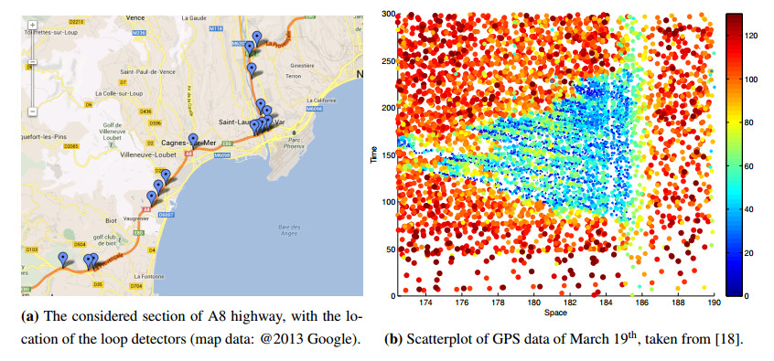
[18] | A. Cabassi, P. Goatin, Validation of traffic flow models on processed GPS data, Research Report RR-8382, INRIA, 2013. |
[19] | Escota (VINCI Autoroutes), accessed: 2019-07-28. Available from: https://corporate.vinci-autoroutes.com/fr/presentation/societes-vinci-autoroutes/escota/en-bref. |
[20] | C. F. Daganzo, The cell transmission model: A dynamic representation of highway traffic consistent with the hydrodynamic theory, Transport. Res. B-Meth., 28 (1994), 269-287. |
[21] | G. F. Newell, A simplified theory of kinematic waves in highway traffic, part II: Queueing at freeway bottlenecks, Transport. Res. B-Meth., 27 (1993), 289-303. |
[22] | S. K. Godunov, A difference method for numerical calculation of discontinuous solutions of the equations of hydrodynamics, Mat. Sb. (N.S.), 47 (1959), 271-306. |
[23] | M. Garavello, B. Piccoli, Traffic flow on networks, volume 1 of AIMS Series on Applied Mathematics, American Institute of Mathematical Sciences (AIMS), Springfield, MO, 2006. Conservation laws models. |
[24] | J.-P. Lebacque, The Godunov scheme and what it means for first order traffic flow models, In Transportation and traffic theory. Proceedings of the 13th international symposium on transportation and traffic theory, Lyon, France, 24-26 JULY 1996, 1996. |
[25] | J. K. Wiens, J. M. Stockie, J. F. Williams, Riemann solver for a kinematic wave traffic model with discontinuous flux, J. Comput. Phys., 242 (2013), 1-23. |
[26] | J. Tryoen, O. Le Maître, A. Ern, Adaptive anisotropic spectral stochastic methods for uncertain scalar conservation laws, SIAM J. Sci. Comput., 34 (2012), A2459-A2481. |
[27] | M. Bulíček, P. Gwiazda, J. Málek, A. Świerczewska-Gwiazda, On scalar hyperbolic conservation laws with a discontinuous flux, Math. Models Methods Appl. Sci., 21 (2011), 89-113. |
[28] | J. a.-P. Dias, M. Figueira, J.-F. Rodrigues. Solutions to a scalar discontinuous conservation law in a limit case of phase transitions, J. Math. Fluid Mech., 7 (2005), 153-163. |
[29] | T. Gimse, Conservation laws with discontinuous flux functions, SIAM J. Math. Anal., 24 (1993), 279-289. |
[30] | E. Cristiani, C. de Fabritiis, B. Piccoli, A fluid dynamic approach for traffic forecast from mobile sensor data, Commun. Appl. Ind. Math., 1 (2010), 54-71. |