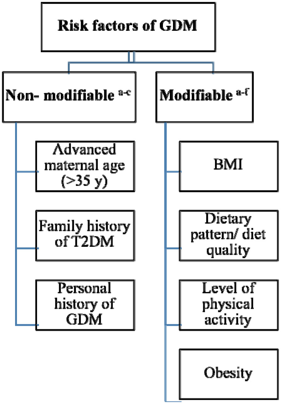
Gestational diabetes mellitus (GDM) is one of the most common metabolic disorders known to develop during pregnancy. Besides obesity and sedentary lifestyles being the main predisposing factors, dietary measures play an important role in its progression too. Hence, managing GDM has become a great challenge for healthcare professionals globally. It is pertinent to establish and manage the predisposing factors for GDM. Many studies have investigated the potential dietary risk factors linked to GDM, especially dietary patterns and diet quality. While certain healthful dietary patterns incorporating wholegrain cereals, high in fruits and vegetables, low meat and saturated fats have been protective against GDM, deficiencies of micronutrients such as potassium, magnesium, and possibly zinc and chromium may predispose one to carbohydrate intolerance. The alterations in iron and zinc body stores could also affect GDM. Dietary iron, vitamin C and D are amongst the micronutrients associated with the development and prevention of diabetes in pregnant women. However, evidences on the effects of vitamins, minerals other indices of maternal diet quality on GDM are inconclusive. This review provides an overview of the emerging evidences on the role of maternal dietary patterns, diet quality and micronutrients, which may contribute in the prevention of GDM across the different economies in the world. The results will empower the healthcare professionals to prevent and manage GDM effectively.
Citation: Snigdha Misra, Yang Wai Yew, Tan Seok Shin. Maternal dietary patterns, diet quality and micronutrient status in gestational diabetes mellitus across different economies: A review[J]. AIMS Medical Science, 2019, 6(1): 76-114. doi: 10.3934/medsci.2019.1.76
Gestational diabetes mellitus (GDM) is one of the most common metabolic disorders known to develop during pregnancy. Besides obesity and sedentary lifestyles being the main predisposing factors, dietary measures play an important role in its progression too. Hence, managing GDM has become a great challenge for healthcare professionals globally. It is pertinent to establish and manage the predisposing factors for GDM. Many studies have investigated the potential dietary risk factors linked to GDM, especially dietary patterns and diet quality. While certain healthful dietary patterns incorporating wholegrain cereals, high in fruits and vegetables, low meat and saturated fats have been protective against GDM, deficiencies of micronutrients such as potassium, magnesium, and possibly zinc and chromium may predispose one to carbohydrate intolerance. The alterations in iron and zinc body stores could also affect GDM. Dietary iron, vitamin C and D are amongst the micronutrients associated with the development and prevention of diabetes in pregnant women. However, evidences on the effects of vitamins, minerals other indices of maternal diet quality on GDM are inconclusive. This review provides an overview of the emerging evidences on the role of maternal dietary patterns, diet quality and micronutrients, which may contribute in the prevention of GDM across the different economies in the world. The results will empower the healthcare professionals to prevent and manage GDM effectively.

| [1] | International Diabetes Federation (2013) IDF Diabetes Atlas (6th Edition) . |
| [2] | Schoenaker DA, Mishra GD, Callaway LK, et al. (2016) The Role of Energy, Nutrients, Foods, and Dietary Patterns in the Development of Gestational Diabetes Mellitus: A Systematic Review of Observational Studies. Diabetes Care ,39: 16-23. |
| [3] | Zhang C, Liu S, Solomon CG, et al. (2006) Dietary fiber intake, dietary glycemic load, and the risk for gestational diabetes mellitus. Diabetes Care ,29: 2223-2230. |
| [4] | Zhang C, Ning Y (2011) Effect of dietary and lifestyle factors on the risk of gestational diabetes: review of epidemiologic evidence. Am J Clin Nutr ,94: 1975S-1979S. |
| [5] | Akhlaghi F, Bagheri SM, Rajabi O (2012) A Comparative Study of Relationship between Micronutrients and Gestational Diabetes. ISRN Obstet Gynecol ,2012: 470419. |
| [6] | Solomon CG, Willett WC, Carey VJ (1997) A prospective study of pregravid determinants of gestational diabetes mellitus. JAMA ,278: 1078-1083. |
| [7] | Bo S, Menato G, Lezo A, et al. (2001) Dietary fat and gestational hyperglycaemia. Diabetologia ,44: 972-978. |
| [8] | Chu SY, Callaghan WM, Kim SY, et al. (2007) Maternal Obesity and Risk of Gestational DIabetes Mellitus. Diabetes Care ,30: 2070-2076. |
| [9] | Saldana TM, Siega-Riz AM, Adair LS (2004) Effect of macronutrient intake on the development of glucose intolerance during pregnancy. Am J Clin Nutr ,79: 479-486. |
| [10] | Wang Y, Storlien LH, Jenkins AB, et al. (2000) Dietary Variables and Glucose Tolerance in Prenancy. Diabetes Care ,23: 460-464. |
| [11] | Krebs-Smith SM (2014) Approaches to Dietary Pattern Analyses: Potential to Inform Guidance. National Cancer Institute, U.S. DEPARTMENT OF HEALTH AND HUMAN SERVICES, National Institute of Health. Nutrition Evidence Library, Technical Expert Collaborative on Study of Dietary Patterns. |
| [12] | Wirt A, Collins CE (2009) Diet quality—what is it and does it matter? Public Health Nutr ,12: 2473-2492. |
| [13] | United Nations (2014) Country Classification. World Economic Situation and Prospects ,143-150. |
| [14] | Zhang C, Schulze MB, Solomon CG, et al. (2006) A prospective study of dietary patterns, meat intake and the risk of gestational diabetes mellitus. Diabetologia ,49: 2604-2613. |
| [15] | Radesky JS, Oken E, Rifas-Shiman SL, et al. (2008) Diet during early pregnancy and development of gestational diabetes. Paediatr Perinat Epidemiol ,22: 47-59. |
| [16] | Morrison MK, Koh D, Lowe JM, et al. (2012) Postpartum diet quality in Australian women following a gestational diabetes pregnancy. Eur J Clin Nutr ,66: 1160-1165. |
| [17] | Tobias DK, Hu FB, Chavarro J, et al. (2012) Healthful dietary patterns and type 2 diabetes mellitus risk among women with a history of gestational diabetes mellitus. Arch Intern Med ,172: 1566-1572. |
| [18] | Tobias DK, Zhang C, Chavarro J, et al. (2012) Prepregnancy adherence to dietary patterns and lower risk of gestational diabetes mellitus. Am J Clin Nutr ,96: 289-295. |
| [19] | Louie JC, Markovic TP, Ross GP, et al. (2013) Higher glycemic load diet is associated with poorer nutrient intake in women with gestational diabetes mellitus. Nutr Res ,33: 259-265. |
| [20] | Lim SY, Yoo HJ, Kim AL, et al. (2013) Nutritional Intake of Pregnant Women with Gestational Diabetes or Type 2 Diabetes Mellitus. Clin Nutr Res ,2: 81-90. |
| [21] | Ferranti EP, Narayan KM, Reilly CM, et al. (2014) Dietary Self-Efficacy Predicts AHEI Diet Quality in Women With Previous Gestational Diabetes. Diabetes Educ ,40: 688-699. |
| [22] | Xiao RS, Simas TA, Person SD, et al. (2015) Diet Quality and History of Gestational Diabetes Mellitus Among Childbearing Women, United States, 2007–2010. Prev Chronic Dis ,12: 140360. |
| [23] | Gresham E, Collins CE, Mishra GD, et al. (2016) Diet quality before or during pregnancy and the relationship with pregnancy and birth outcomes: The Australian Longitudinal Study on Women's Health. Public Health Nutr ,19: 2975-2983. |
| [24] | Meinilä J, Valkama A, Koivusalo SB, et al. (2016) Healthy Food Intake Index (HFII) - Validity and reproducibility in a gestational-diabetes-risk population. BMC Public Health ,16: 680. |
| [25] | de Seymour J, Chia A, Colega M, et al. (2016) Maternal dietary patterns and gestational diabetes mellitus in a multi-ethnic Asian cohort: The GUSTO study. Nutrients ,8: 574. |
| [26] | Gicevic S, Gaskins AJ, Fung TT, et al. (2018) Evaluating pre-pregnancy dietary diversity vs. dietary quality scores as predictors of gestational diabetes and hypertensive disorders of pregnancy. PLoS One ,13: e0195103. |
| [27] | Nascimento GR, Alves LV, Fonseca CL, et al. (2016) Dietary patterns and gestational diabetes mellitus in a low-income pregnant women population in Brazila—A cohort study. Arch Latinoam Nutri ,66: 301-308. |
| [28] | Izadi V, Tehrani H, Haghighatdoost F, et al. (2016) Adherence to the DASH and Mediterranean diets is associated with decreased risk for gestational diabetes mellitus. Nutrition ,32: 1092-1096. |
| [29] | Sedaghat F, Akhoondan M, Ehteshami M, et al. (2017) Maternal Dietary Patterns and Gestational Diabetes Risk: A Case-Control Study. J Diabetes Res ,2017: 5173926. |
| [30] | Zareei S, Homayounfar R, Naghizadeh MM, et al. (2018) Dietary pattern in pregnancy and risk of gestational diabetes mellitus (GDM). Diabetes Metab Syndr ,12: 399-404. |
| [31] | Sahariah SA, Potdar RD, Gandhi M, et al. (2016) A Daily Snack Containing Leafy Green Vegetables, Fruit, and Milk before and during Pregnancy Prevents Gestational Diabetes in a Randomized, Controlled Trial in Mumbai, India. J Nutr ,146: 1453S-1460S. |
| [32] | Lao TT, Chan PL, Tam KF (2001) Gestational diabetes mellitus in the last trimester - A feature of maternal iron excess? Diabet Med ,18: 218-223. |
| [33] | Lao TT, Ho LF (2004) Impact of iron deficiency anemia on prevalence of gestational diabetes mellitus. Diabetes Care ,27: 650-656. |
| [34] | Chan KKL, Chan BCP, Lam KF, et al. (2009) Iron supplement in pregnancy and development of gestational diabetes—A randomised placebo-controlled trial. BJOG: Int J Obstet Gy ,116: 789-797. |
| [35] | Bo S, Menato G, Villois P, et al. (2009) Iron supplementation and gestational diabetes in midpregnancy. Am J Obstet Gynecol ,201: 158.e1-158.e6. |
| [36] | Bowers K, Yeung E, Williams MA, et al. (2011) A prospective study of prepregnancy dietary iron intake and risk for gestational diabetes mellitus. Diabetes Care ,34: 1557-1563. |
| [37] | Qiu C, Zhang C, Gelaye B, et al. (2011) Gestational diabetes mellitus in relation to maternal dietary heme iron and nonheme iron intake. Diabetes Care ,34: 1564-1569. |
| [38] | Helin A, Kinnunen TI, Raitanen J, et al. (2012) Iron intake, haemoglobin and risk of gestational diabetes: A prospective cohort study. BMJ Open ,2: e001730. |
| [39] | Darling AM, Mitchell AA, Werler MM (2016) Preconceptional iron intake and gestational diabetes mellitus. Int J Environ Res Public Health ,13: 525. |
| [40] | Bo S, Lezo A, Menato G, et al. (2005) Gestational hyperglycemia, zinc, selenium, and antioxidant vitamins. Nutrition ,21: 186-191. |
| [41] | Nabouli MR, Lassoued L, Bakri Z, et al. (2016) Modification of Total Magnesium level in pregnant Saudi Women developing gestational diabetes mellitus. Diabetes Metab Syndr ,10: 183-185. |
| [42] | Zhang C, Qiu C, Hu FB, et al. (2008) Maternal plasma 25-hydroxyvitamin D concentrations and the risk for gestational diabetes mellitus. PLoS One ,3: e3753. |
| [43] | Makgoba M, Nelson SM, Savvidou M, et al. (2011) First-trimester circulating 25-hydroxyvitamin D levels and development of gestational diabetes mellitus. Diabetes Care ,34: 1091-1093. |
| [44] | Baker AM, Haeri S, Camargo CA, et al. (2012) First-trimester maternal vitamin D status and risk for gestational diabetes (GDM) a nested case-control study. Diabetes Metab Res Rev ,28: 164-168. |
| [45] | Burris HH, Rifas-Shiman SL, Kleinman K, et al. (2012) Vitamin D deficiency in pregnancy and gestational diabetes mellitus. Am J Obstet Gynecol ,207: 182.e1-182.e8. |
| [46] | Whitelaw DC, Scally AJ, Tuffnell DJ, et al. (2014) Associations of circulating calcium and 25-hydroxyvitamin D with glucose metabolism in pregnancy: A cross-sectional study in European and south Asian women. J Clin Endocrinol Metab ,99: jc20132896. |
| [47] | Arnold DL, Enquobahrie DA, Qiu C, et al. (2015) Early Pregnancy Maternal Vitamin D Concentrations and Risk of Gestational Diabetes Mellitus. Paediatr Perinat Epidemiol ,29: 200-210. |
| [48] | Wolak T, Sergienko R, Wiznitzer A, et al. (2010) Low potassium level during the first half of pregnancy is associated with lower risk for the development of gestational diabetes mellitus and severe pre-eclampsia. J Matern Fetal Neonatal Med ,23: 994-998. |
| [49] | Wolak T, Shoham-Vardi I, Sergienko R, et al. (2016) High potassium level during pregnancy is associated with future cardiovascular morbidity. Journal Matern Fetal Neonatal Med ,29: 1021-1024. |
| [50] | Gunton JE, Hams G, Hitchman R, et al. (2001) Serum chromium does not predict glucose tolerance in late pregnancy. Am J Clin Nutr ,73: 99-104. |
| [51] | Houldsworth A, Williams R, Fisher AS, et al. (2017) Proposed Relationships between the Degree of Insulin Resistance, Serum Chromium Level/BMI and Renal Function during Pregnancy and the Pathogenesis of Gestational Diabetes Mellitus. Int J Endocrinol Metab Disord ,3: 1-8. |
| [52] | Zhang C, Williams MA, Sorensen TK, et al. (2004) Maternal plasma ascorbic acid (vitamin C) and risk of gestational diabetes mellitus. Epidemiology ,15: 597-604. |
| [53] | Afkhami-Ardekani M, Rashidi M (2009) Iron status in women with and without gestational diabetes mellitus. J Diabetes Complications ,23: 194-198. |
| [54] | Amiri FN, Basirat Z, Omidvar S, et al. (2013) Comparison of the serum iron, ferritin levels and total iron-binding capacity between pregnant women with and without gestational diabetes. J Nat Sci Biol Med ,4: 302-305. |
| [55] | Behboudi-Gandevani S, Safary K, Moghaddam-Banaem L, et al. (2013) The relationship between maternal serum iron and zinc levels and their nutritional intakes in early pregnancy with gestational diabetes. Biol Trace Elem Res ,154: 7-13. |
| [56] | Javadian P, Alimohamadi S, Gharedaghi MH, et al. (2014) Gestational diabetes mellitus and iron supplement; effects on pregnancy outcome. Acta Med Iran ,52: 385-389. |
| [57] | Wang Y, Tan M, Huang Z, et al. (2002) Elemental Contents in Serum of Pregnant Women with Gestational Diabetes Mellitus. Biol Trace Elem Res ,88: 113-118. |
| [58] | Hussein HK (2005) Level of serum copper and zinc in pregnant women with gestational diabetes mellitus. J Fac Med Baghdad ,47: 287-289. |
| [59] | Roshanravan N, Alamdari NM, Ghavami A, et al. (2017) Serum levels of copper, zinc and magnesium in pregnant women with Impaired Glucose Tolerance test: a case-control study. Prog Nutr ,20: 1-5. |
| [60] | Behrashi M, Mahdian M, Aliasgharzadeh A (2011) Effects of zinc supplementation on glycemic control and complications of gestational diabetes. Pak J Med Sci ,27: 1203-1206. |
| [61] | Genova MP, Atanasova B, Todorova-Ananieva K (2014) Plasma and Intracellular Erythocyte Zinc Levels during Pregnancy in Bulgarian Females with and without Gestational Diabetes. Int J Adv Res ,2: 661-667. |
| [62] | Roshanravan N, Alizadeh M, Hedayati M, et al. (2015) Effect of zinc supplementation on insulin resistance, energy and macronutrients intakes in pregnant women with impaired glucose tolerance. Iran J Public Health ,44: 211-217. |
| [63] | Karamali M, Heidarzadeh Z, Seifati SM, et al. (2015) Zinc supplementation and the effects on metabolic status in gestational diabetes: A randomized, double-blind, placebo-controlled trial. J Diabetes Complications ,29: 1314-1319. |
| [64] | Genova MP, Atanasova B, Todorova-Ananieva K, et al. (2016) Zinc and Insulin Resistance in Pregnancy Complicated with Gestational Diabetes. Int J Health Sci Res ,6: 191-197. |
| [65] | Parast VM, Paknahad Z (2017) Antioxidant Status and Risk of Gestational Diabetes Mellitus: a Case-Control Study. Clin Nutr Res ,6: 81-88. |
| [66] | Genova MP, Todorova-Ananieva K, Atanasova B (2014) Plasma and Intracellular Erythrocyte Magnesium Levels in Healthy Pregnancy and Pregnancy with Gestational Diabetes. Int J Sci Res ,3: 326-329. |
| [67] | Asemi Z, Jamilian M, Mesdaghinia E, et al. (2015) Effects of selenium supplementation on glucose homeostasis, inflammation, and oxidative stress in gestational diabetes: Randomized, double-blind, placebo-controlled trial. Nutrition ,31: 1235-1242. |
| [68] | Mostafavi E, Nargesi AA, Asbagh FA, et al. (2015) Abdominal obesity and gestational diabetes: The interactive role of magnesium. Magnes Res ,28: 116-125. |
| [69] | Goker Tasdemir U, Tasdemir N, Kilic S, et al. (2015) Alterations of ionized and total magnesium levels in pregnant women with gestational diabetes mellitus. Gynecol Obstet Invest ,79: 19-24. |
| [70] | Karamali M, Bahramimoghadam S, Sharifzadeh F, et al. (2018) Magnesium-zinc-calcium-vitamin D co-supplementation improves glycemic control and markers of cardio-metabolic risk in gestational diabetes: a randomized, double-blind, placebo-controlled trial. Appl Physiol Nutr Metab ,43: 565-570. |
| [71] | Maktabi M, Jamilian M, Amirani E, et al. (2018) The effects of magnesium and vitamin E co-supplementation on parameters of glucose homeostasis and lipid profiles in patients with gestational diabetes. Lipids Health Dis ,17: 163. |
| [72] | Tan M, Sheng L, Qian Y, et al. (2001) Changes of serum selenium in pregnant women with gestational diabetes mellitus. Biol Trace Elem Res ,83: 231-237. |
| [73] | Kilinc M, Guven MA, Ezer M, et al. (2008) Evaluation of serum selenium levels in Turkish women with gestational diabetes mellitus, glucose intolerants, and normal controls. Biol Trace Elem Res ,123: 35-40. |
| [74] | Asemi Z, Jamilian M, Esmaillzadeh A, et al. (2014) Effects of calcium-vitamin D co-supplementation on glycaemic control, inflammation and oxidative stress in gestational diabetes: A randomised placebo-controlled trial. Diabetologia ,57: 1798-1806. |
| [75] | Zhang Q, Cheng Y, He M, et al. (2016) Effect of various doses of vitamin D supplementation on pregnant women with gestational diabetes mellitus: A randomized controlled trial. Exp Ther Med ,12: 1889-1895. |
| [76] | Jamilian M, Samimi M, Ebrahimi FA, et al. (2017) The effects of vitamin D and omega-3 fatty acid co-supplementation on glycemic control and lipid concentrations in patients with gestational diabetes. J Clin Lipidol ,11: 459-468. |
| [77] | Prasad DKV, Sheela P, Kumar AN, et al. (2013) Iron Levels Increased in Serum from Gestational Diabetes Mellitus Mothers in Coastal Area of Andhra Pradesh. J Diabetes Metab ,4: 269. |
| [78] | Joseph M, Das Gupta R, Shetty S, et al. (2017) How Adequate are Macro- and Micronutrient Intake in Pregnant Women with Diabetes Mellitus? A Study from South India. J Obstet Gynecol India ,68: 400-407. |
| [79] | Hamdan HZ, Elbashir LM, Hamdan SZ, et al. (2014) Zinc and selenium levels in women with gestational diabetes mellitus at Medani Hospital, Sudan. J Obstet Gynaecol ,34: 567-570. |
| [80] | Asha D, Nivedita N, Daniel M, et al. (2014) Association of serum copper level with fasting serum glucose in south Indian women with gestational diabetes mellitus. Int J Clin Exp Physiol ,1: 298-302. |
| [81] | Sundararaman PG, Sridhar GR, Sujatha V, et al. (2012) Serum chromium levels in gestational diabetes mellitus. Indian J Endocrinol Metab ,16: S70-S73. |
| [82] | Muthukrishnan J, Dhruv G (2015) Vitamin D status and gestational diabetes mellitus. Indian J Endocrinol Metab ,19: 616-619. |
| [83] | Krishnaveni GV, Hill JC, Veena SR, et al. (2009) Low plasma vitamin B12 in pregnancy is associated with gestational ‘diabesity’ and later diabetes. Diabetologia ,52: 2350-2358. |
| [84] | Mishu FA, Muttalib MA, Sultana B (2018) Serum Zinc and Copper Levels in Gestational Diabetes Mellitus in a Tertiary Care Hospital of Bangladesh. Birdem Med J ,8: 52-55. |
| [85] | American Diabetes Association (2018) Management of Diabetes in Pregnancy: Standards of Medical Care in Diabetes. Diabetes Care ,41: S137-S143. |
| [86] | Esmaillzadeh A, Azadbakht L, Kimiagar M (2007) Dietary Pattern Analysis: A New Approach to Identify Diet-disease Relations. Iran J Nutr Sci Food Technol ,2: 71-80. |
| [87] | Rashidkhani B, Shaneshin M, Neyestani T, et al. (2009) Validity of energy intake reporting and its association with dietary patterns among 18–45-year old women in Tehran. Iran J Nutr Sci Food Technol ,4: 63-74. |
| [88] | Green R, Milner J, Joy EJ, et al. (2016) Dietary patterns in India: a systematic review. Br J Nutr ,116: 142-148. |
| [89] | Mazzocchi M, Brasili C, Sandri E (2008) Trends in dietary patterns and compliance with World Health Organization recommendations: A cross-country analysis. Public Health Nutr ,11: 535-540. |
| [90] | Catalano PM, McIntyre HD, Cruickshank JK, et al. (2012) The hyperglycemia and adverse pregnancy outcome study: Associations of GDM and obesity with pregnancy outcomes. Diabetes Care ,35: 780-786. |
| [91] | Genova M, Atanasova B, Ivanova I, et al. (2018) Trace Elements and Vitamin D in Gestational Diabetes. Acta Med Bulgarica ,45. |
| [92] | Fu S, Li F, Zhou J, et al. (2016) The Relationship Between Body Iron Status, Iron Intake and Gestational Diabetes. Medicine ,95: e2383. |
| [93] | Fernández-Real JM, McClain D, Manco M (2015) Mechanisms Linking Glucose Homeostasis and Iron Metabolism Toward the Onset and Progression of Type 2 Diabetes. Diabetes Care ,38: 2169-2176. |
| [94] | Moghaddam-banaem L (2017) Maternal Serum Iron and Zinc Levels and Gestational Diabetes. Arch Med Lab Sci ,3: 28-33. |
| [95] | Kong FJ, Ma LL, Chen SP, et al. (2016) Serum selenium level and gestational diabetes mellitus: a systematic review and meta-analysis. Nutr J ,15: 94. |
| [96] | Chehade JM, Sheikh-Ali M, Mooradian AD (2009) The Role of Micronutrients in Managing Diabetes. Diabetes Spectrum ,22: 214-218. |
Figures(1) / Tables(7)

Snigdha Misra, Yang Wai Yew, Tan Seok Shin. Maternal dietary patterns, diet quality and micronutrient status in gestational diabetes mellitus across different economies: A review[J]. AIMS Medical Science, 2019, 6(1): 76-114. doi: 10.3934/medsci.2019.1.76


 DownLoad: