


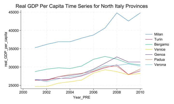
Figure 1.
Time series of the outcome variable in North Italy provinces.
Motivated by some ordinary and extreme connectedness properties of topologies, we introduce several reasonable connectedness properties of relators (families of relations). Moreover, we establish some intimate connections among these properties.
More concretely, we investigate relationships among various minimalness (well-chainedness), connectedness, hyper- and ultra-connectedness, door, superset, submaximality and resolvability properties of relators.
Since most generalized topologies and all proper stacks (ascending systems) can be derived from preorder relators, the results obtained greatly extends some standard results on topologies. Moreover, they are also closely related to some former results on well-chained and connected uniformities.
Citation: Muwafaq Salih, Árpád Száz. Generalizations of some ordinary and extreme connectedness properties of topological spaces to relator spaces[J]. Electronic Research Archive, 2020, 28(1): 471-548. doi: 10.3934/era.2020027
| [1] | Mahinur Begum Mimi, Md. Ahasan Ul Haque, Md. Golam Kibria . Does human capital investment influence unemployment rate in Bangladesh: a fresh analysis. National Accounting Review, 2022, 4(3): 273-286. doi: 10.3934/NAR.2022016 |
| [2] | Van Hoa Tran, Quang Thao Pham . Growth and poverty reduction in Vietnam: A strategic policy modelling study. National Accounting Review, 2024, 6(3): 449-464. doi: 10.3934/NAR.2024020 |
| [3] | Kewei Ma, Guido Ferrari, Zichuan Mi . SAM-based analysis of China’s economic system and measurement of the effects of a VAT rate cut after the tax reform. National Accounting Review, 2020, 2(1): 26-52. doi: 10.3934/NAR.2020002 |
| [4] | Sylvie Kotíková . Spillover effects: A challenging public interest to measure. National Accounting Review, 2023, 5(4): 373-404. doi: 10.3934/NAR.2023022 |
| [5] | Joana Cobbinah, Tan Zhongming, Albert Henry Ntarmah . Banking competition and stability: evidence from West Africa. National Accounting Review, 2020, 2(3): 263-284. doi: 10.3934/NAR.2020015 |
| [6] | Mustafa Tevfik Kartal . Do activities of foreign investors affect main stock exchange indices? Evidence from Turkey before and in time of Covid-19 pandemic. National Accounting Review, 2020, 2(4): 384-401. doi: 10.3934/NAR.2020023 |
| [7] | Ragnar Nymoen . Economic Covid-19 effects analysed by macro econometric models—the case of Norway. National Accounting Review, 2023, 5(1): 1-22. doi: 10.3934/NAR.2023001 |
| [8] | Giorgio Colacchio, Anna Serena Vergori . GDP growth rate, tourism expansion and labor market dynamics: Applied research focused on the Italian economy. National Accounting Review, 2022, 4(3): 310-328. doi: 10.3934/NAR.2022018 |
| [9] | Jawad Saleemi . COVID-19 and liquidity risk, exploring the relationship dynamics between liquidity cost and stock market returns. National Accounting Review, 2021, 3(2): 218-236. doi: 10.3934/NAR.2021011 |
| [10] | Vladimir Hlasny . Social assistance and workers' long-term well-being in Egypt. National Accounting Review, 2023, 5(2): 174-185. doi: 10.3934/NAR.2023011 |
Motivated by some ordinary and extreme connectedness properties of topologies, we introduce several reasonable connectedness properties of relators (families of relations). Moreover, we establish some intimate connections among these properties.
More concretely, we investigate relationships among various minimalness (well-chainedness), connectedness, hyper- and ultra-connectedness, door, superset, submaximality and resolvability properties of relators.
Since most generalized topologies and all proper stacks (ascending systems) can be derived from preorder relators, the results obtained greatly extends some standard results on topologies. Moreover, they are also closely related to some former results on well-chained and connected uniformities.
In recent years, Europe has seen a significant rise in the construction of numerous "next-generation stadiums". As proposed by the globally renowned architectural and design firm Populous1, a "next generation stadium" refers to a state-of-the-art sports and entertainment venue that leverages advanced technologies, sustainable infrastructure, and fan-centric designs to enhance functionality and the overall experience. These stadiums are characterized by features such as high-speed connectivity (e.g., 5G networks and Wi-Fi for internet access and interactive fan engagement), renewable energy systems, flexible multi-use spaces, and immersive digital platforms. This new type of stadium places significant emphasis on the fan experience by incorporating club stores, hotels, restaurants, and other facilities directly within the stadium structure. Additionally, these projects often involve the renewal or, where necessary, the construction of transport networks to ensure seamless accessibility and connectivity for fans. The best example of these "next-generation stadiums" is the Tottenham Hotspur Stadium (London, UK), which opened in 2019. This multi-use stadium is equipped with heated seats, a glass tunnel for fans to see players up close, and unique acoustics that amplify crowd noise. In addition to hosting football matches, the stadium also includes restaurants, retail outlets, and a skywalk terrace for fans.
This stadium is the first purposefully built stadium for NFL games outside the U.S., featuring a retractable natural turf pitch that slides under the South Stand in just 25 minutes, revealing an artificial playing surface. This allows American football to take place during the Premier League football season without affecting the quality of the natural turf pitch. The stadium now hosts two regular season NFL games each year as part of an ongoing partnership between the league and Tottenham Hotspur. The adaptability of the stadium has allowed it to host some of the biggest events in sports and entertainment, from a world heavyweight boxing title clash between Anthony Joshua and Oleksandr Usyk in 2022 to five sellout Beyoncé concerts in 2023. This new project has generated approximately 3,500 jobs during its construction phase, highlighting its significant contribution to local employment. Additionally, the average revenue per game has increased substantially, reaching €7 million compared to the €1 million generated by the previous version of the stadium. This remarkable growth underscores the economic impact of transitioning to a next-generation stadium model2.The latest example of a next-generation stadium is the Santiago Bernabéu (Madrid), with an estimated cost of €800 million. Among its numerous innovations is a retractable pitch, costing nearly €250 million, which ensures that players always compete on a perfect playing surface.
2https://www.calcioefinanza.it/2024/04/06/football-affairs-incasso-stadio-tottenham/?refresh_ce.
These are just the most illustrious examples; however, over the past 15 years, numerous next-generation stadiums have been built across Europe, such as the Wanda Metropolitano of Atlético Madrid in 2017, the Puskás Aréna in Budapest in 2019, and the Parken Stadium in Copenhagen in 2020. Surprisingly, none of these constructions have been studied to evaluate their economic impact. In Italy, several teams such as Roma, Inter, and Milan have presented projects for this new type of stadium, but so far, the only team that has successfully built one is Juventus. In the city of Turin, after announcing the stadium in September 2008, they inaugurated it in September 2011.
The pioneering study on the economic effects of professional sports was conducted by Baade and Dye (1998). It analyzed the impact of professional sports on annual manufacturing employment, real value added in manufacturing, and new capital expenditures by manufacturing firms across eight metropolitan areas from 1965 to 1978.
The data used for the analysis are from the Annual Survey of Manufactures, with regressors including the population of the metropolitan area (MA), a time trend, and indicators for the presence of new or renovated stadiums, professional football franchises, and professional baseball franchises. The findings revealed limited evidence that variations in professional sports facilities (or franchises) significantly influenced employment, value added, or capital expenditures. Among the franchise/facility indicators, only four parameters were statistically significant at the 5% level, with three showing positive effects and one showing a negative effect.
Baade and Tiehen (1990) extended their analysis to examine the economic impact of professional sports on annual real metropolitan area (MA) personal income and the ratio of MA personal income to regional personal income across nine metropolitan areas between 1965 and 1983. Utilizing the same explanatory variables as their earlier study, the authors found no evidence to suggest that the presence of sports franchises or facilities accounted for differences in real personal income among metropolitan areas.
Baade (1996) continued this line of research by examining the impact of professional sports on real per capita income and the metropolitan area's share of state employment in the Amusement and Recreation industry and the Commercial Sports industry. This analysis covered 48 metropolitan areas between 1957 and 1989, including cities with and without professional sports teams. The dependent variable, real per capita income, was transformed using a complex function of the average per capita income level across the sample cities and first differences. Separate regressions were estimated for each metropolitan area, with explanatory variables including the number of sports franchises and the number of sports facilities less than ten years old. Findings showed that the sports facility and franchise variables were generally not statistically significant, and when they were, no consistent pattern in the signs of the coefficients emerged.
Baade (1996) concluded that professional sports franchises or facilities did not have a positive impact on real per capita income or employment in the relevant industry classifications. Baade and Sanderson (1997) investigated the employment effects of sports facilities using data from the Amusements and Recreation and Commercial Sports industry classifications of the Standard Industrial Classification (SIC) for ten cities and their respective states over the period from 1958–1993. Separate regressions were estimated for each city, with the dependent variable being the city's share of state employment in either the Amusements and Recreation or Commercial Sports industries. They found minimal evidence that newly constructed stadiums or additional professional teams significantly influenced employment shares.
Miller (2002) investigated the impact of two professional sports facility construction projects on construction industry employment in St. Louis, MO. The empirical models incorporated controls for factors influencing construction industry employment and accounted for the effects of wages on employment levels. Sports-related variables were included as indicators for the specific quarters during which the Kiel Center and TransWorld Dome were under construction. The findings showed that the construction of these sports facilities had no statistically significant effect on construction industry employment. These results challenge the claims made in promotional economic impact studies, which often assert that building sports facilities will lead to substantial increases in urban employment. Coates and Humphreys (2008) demonstrated that in the U.S., in the long term, there is no justification for public funding of large stadium construction projects. Their analysis revealed that such investments fail to generate the economic growth often promised by proponents. Authors offer an argument against sports subsidies based on economic intuition, survey evidence that a majority of economists believe that sports subsidies are unwarranted, and a review of the existing literature on the economic impact of professional sports.
Instead, Santo (2005), in his study, showed that in the United States, the construction of new football and baseball stadiums is positively correlated with the growth of various economic variables in the metropolitan area where the stadium is built.
There are two main points to consider regarding these studies: The first is that they do not focus on observing the effects of the construction of next-generation stadiums but rather on the effects of building general sports facilities (such as new stadiums that do not qualify as next-generation or other sports fields). The second is that these papers predominantly use OLS regressions as their econometric technique, which, if a relationship is present, can only identify mere correlation without providing any evidence of causality.
The objective of this article is to provide, for the first time, a causal interpretation of the change in the well-being of citizens in the metropolitan area where a next-generation stadium was built.
To achieve this, the synthetic control method (SCM), an econometric technique developed by Abadie et al. (2010), was employed. Unlike OLS regression, SCM allows for a causal interpretation rather than a mere correlation. In this study, the application of SCM enables a comparison between the real GDP per capita trajectory of the city of Turin, where the stadium was constructed, and the hypothetical GDP per capita trajectory that would have occurred in the absence of the stadium. The counterfactual is derived through a dual minimization problem that selects a weighted combination of control units to best replicate the pre-treatment characteristics of Turin. This approach not only highlights the potential causal impact of the stadium construction on the economic well-being of the metropolitan area but also contributes to the broader understanding of the implications of next-generation sports facilities on urban economies. Another advantage of using this method is the transparency of the fit, as it is possible to observe the weight assigned to each province in creating the synthetic control.
However, this study has limited external validity since the results are based on a treatment group consisting of only one Italian province (Turin). As a consequence, it is not possible to determine whether the findings can be generalized or if they are specific to Turin. In the coming years, as new stadiums are constructed in other Italian provinces such as Rome and Milan, future studies will have the opportunity to confirm or refute the findings presented here. This will help determine whether the results can be generalized or remain specific to Turin.
The data used in this study consist of a panel of 18 Italian provinces, capturing economic and social variables such as the real GDP per capita, employment rate, net exports, and net registration rate, observed over the period from 2001 to 2016.
The findings highlight a short-term positive impact of the stadium's construction on the well-being of Turin's citizens, with an approximate 2% increase in real GDP per capita. However, this was followed by a modest spring-back effect, as the GDP fell below the synthetic control level by around 1% in the year after the stadium's completion. Interestingly, the study also reveals a small positive short-term impact of the stadium's construction announcement on the real GDP per capita of Turin's residents. This effect is likely attributable to a shift in investor expectations, as the announcement of the stadium project may have spurred early investments in the area. Lastly, from 2013 to 2016 (the final years considered in this study), there appears to be a positive modest structural economic effect of the treatment (Juventus Stadium construction) on the well-being of Turin's citizens. During this period, the observed real GDP per capita trajectory consistently remains higher than the counterfactual in each year.
The rest of this paper is structured as follows: Section 2 reports data selection, variables of interest, and data validation, and section 3 presents the econometric strategy. Section 4 empirically explores the economic impact of the Juventus Stadium on the well-being of inhabitants of Turin. Section 5 concludes the article.
As previously discussed, there are two crucial steps for creating a robust synthetic control. The first is the selection of the treatment episodes. This is relatively straightforward in our case, as the only episode in Italy involving the construction of a next-generation stadium is the Juventus Stadium in 2011 (Turin). The second step is determining which provinces should form the control group, to which the algorithm will be applied to identify the weights that—once assigned to the untreated provinces—will provide the synthetic control of Turin.
The initial dataset consists of the following provinces: Bergamo, Bologna, Cagliari, Catania, Florence, Genoa, Milan, Naples, Padua, Palermo, Parma, Perugia, Prato, Reggio Emilia, Rome, Turin, Venice, and Verona. For these provinces, time series data from 2001 to 2016 were observed for the following variables: real GDP per capita pre- and post-treatment, exports and imports in euros, employment rate, number of patents registered per year (as a proxy for research and development), and the net business registration rate. These variables were chosen because, according to the literature (Blomstrom et al., 1992; Ilter, 2017; Formánek, 2019), they are the ones that contribute the most to explaining real GDP per capita.
Provinces have been selected for the control group based on:
1. Similarity in pre-treatment characteristics (outcome and regressors);
2. Exclusion of treated units;
3. Exclusion of units with structural differences;
4. Data avability and quality.
To compare the real GDP per capita time series of Turin before the treatment with those of other provinces, the eighteen provinces have been divided into three distinct geographical groups3:
3The subdivision does not correspond to the one provided by Italian National Institute of Statistics (ISTAT).
● North Italy Provinces: Bergamo, Genoa, Milan, Padua, Venice, and Verona;
● Center Italy Provinces: Bologna, Florence, Parma, Perugia, Prato, Reggio nell'Emilia, and Rome;
● South Italy Provinces: Cagliari, Catania, Naples, and Palermo.
As shown by Figure 1 within North Italy provinces only Milan's outcome has a very different distribution and it can be excluded from the donor pool.
Instead, Figure 2 shows that Rome's and Perugia's levels of real GDP per capita are very far from the one of Turin and both can be excluded from the donor pool.

Lastly, observing Figure 3 we can conclude that all the South Italy provinces can be excluded from the donor pool since their real GDP per capita time series is very different (in terms of level and movement) from the one of Turin.

For those interested in further details on the exclusion of the cities of Milan, Catania, Cagliari, Naples, Palermo, Perugia, and Rome from the donor pool, descriptive statistics for all provinces are available in the Table 3.
According to the literature (Firpo and Possebom, 2018; Kreif et al., 2016), an additional step could be to use cluster analysis. Cluster analysis is a statistical technique used to group a set of objects into clusters or groups based on their similarities. The goal is to ensure that objects within the same cluster are more similar to each other than to those in other clusters. In this analysis, only the provinces that belong to the same cluster as Turin in the donor pool have been retained. As suggested by Wu (2012), the use of k-means is preferable if there is a clear idea of the number of clusters and if data do not present outliers (since it minimizes the variance within clusters, it is sensitive to outliers) as in this study case.
The k-means clustering process works in this way:
1. Initialization: Begin by randomly selecting K points from the dataset to serve as the initial cluster centroids.
2. Assignment: For each data point, compute its distance to each of the K centroids and assign it to the cluster with the nearest centroid. This step forms K distinct clusters.
3. Update centroids: After assigning all data points, update the centroids by calculating the mean of the points within each cluster.
4. Iteration: Repeat the assignment and update steps until convergence. Convergence occurs when the centroids stabilize or after a set number of iterations.
5. Final output: Once converged, the algorithm provides the final centroids and the cluster assignment for each data point.
Applying the process just described to our dataset yields the following two clusters:
● Cluster 1: Bergamo, Genoa, Padua, Parma, and Venice;
● Cluster 2: Bologna, Florence, Prato, Reggio nell'Emilia, Turin, and Verona.
As previously stated, Bologna, Florence, Prato, Reggio nell'Emilia, and Verona will be part of the donor pool. The algorithm once applied to the control group gives the following weights:
| Province | Weight |
| Bologna | 0.3 |
| Florence | 0 |
| Perugia | 0.581 |
| Prato | 0 |
| Reggio nell'Emilia | 0.119 |
| Verona | 0 |
 DownLoad:
CSV
DownLoad:
CSV
The synthetic control method (SCM), introduced by Abadie and Gardeazabal (2003) and further refined by Abadie et al. (2010), offers a useful approach for comparative case studies, particularly in assessing the economic effects of building next-generation stadiums. The synthetic control method constructs a weighted synthetic control group that mimics the key characteristics of the treated province. After the construction of the stadium, SCM estimates the counterfactual outcome by comparing the post-intervention trajectory of the treated province with that of its synthetic counterpart. In a formal sense, it is helpful to frame the discussion in terms of potential outcomes within a panel data structure.
Suppose we observe a panel of I+1 provinces over T periods. Only province i is treated (experience the stadium construction) at time T0, with T0<T, while the remaining I provinces remain untreated being part of the control group. The treatment effect for province i at time t is defined as:
| τi,t=Yi,t(1)−Yi,t(0)=Yi,t−Yi,t(0) | (1) |
where Yi,t(1) and Yi,t(0) stand for the potential outcome with and without treatment, respectively. The estimand of interest is the vector (τi,T0+1,...,τi,T).
While the potential outcome Yi,t(1) is observable and corresponds to Yi,t, Yi,t(0), representing the counterfactual, cannot be observed.
Abadie et al. (2010) demonstrated how to estimate the aforementioned treatment effects by applying the following general model to the potential outcomes for all units:
| Yj,t(0)=γt+vj,t | (2) |
| Yj,t(1)=τj,t+γt+vj,t | (3) |
with j = 1, ..., I+1.
τj,t is different from zero only when j = i and t≥T0. It can be noticed that both potential outcomes depend on common factor γt and error vj,t which can be rewritten as:
| vj,t=θtZi+λtμj+ϵj,t | (4) |
where Zj represents that characteristic of units j that we actually observe, μj represents the characteristics of unit j that we do not observe, and θt and λt are vectors of time-specific parameters. Lastly, ϵj,t is the individual transitory shock (random noise). Something very relevant is that in order to approximate the outcome trajectory for the treated unit, T0 has to be large and the variance of Y has to be not too large. Settings with small T0 or large noise create substantial risk of over-fitting. In our framework, since all elements in Zj (real GDP per capita values in the pre-treatment period, unemployment rate, net enterprise enrollment rate, current account balance, number of patents per year) refer to the pre-stadium period, and the assumption that they are unaffected by the treatment implies that we exclude any anticipatory effects.
Card and Krueger (1993) were the first to discuss in an empirical work the anticipatory effect, which refers to the behavioral changes that occur before an expected event or intervention, based on the anticipation of future policy or treatment. Essentially, individuals, firms, or other entities adjust their actions in advance of a known or expected change, which can influence the outcomes researchers aim to measure. In order to control for that, a dummy variable been created that assumes "1" from the year of the stadium announcement (2008) and "0" before.
Define W=(w1,…,wi)′ as a (I×1) vector of weights such that wj ≥0 for j=1,2,…,i and ∑wj=1 (to avoid extrapolation).
Let X1 be a (k×1) vector of pre-intervention characteristics for the treated unit and let X0 be a (k×j) matrix which contains the same variables for the unaffected units.
Vector W∗=(w∗1,…,w∗i)′ is chosen to minimize the discrepancy between characteristics:
‖X1−X0W‖ = (∑kn=1vn(xn,1−w2Xn,2−⋯−wiXn,i)2)1/2, where vn are positive constants that reflect the predictive power of each of the k predictors.
This method solves a dual optimization problem:
1. Weights optimization:
| minw(Xtreated−Xuntreatedw)′V(Xtreated−Xuntreatedw) | (5) |
where V is a weighting matrix. The minimization process is carried out by selecting appropriate weights in order to understand which province (and how much) to consider in the analysis.
2. Variables optimization:
| minV(Ytreated−Yuntreatedw∗(V))′(Ytreated−Yuntreatedw∗(V)) | (6) |
Minimization is done over the weighting matrix such that the outcome of the synthetic control is as similar as possible to the one of the treated province. The matrix V assigns weights to the characteristics (regressors) to best predict the outcome variable. Let Yj,t be the value for unit j at time t. For a post-intervention period (t≥T0), an unbiased estimator of the treatment effect is: ^τi,t=Yi,t−∑Ij=1w∗jYj,t.
In order to obtain a good synthetic control, structural similarities between groups and common pre-trends are needed.
In essence, the synthetic control algorithm estimates the missing counterfactual by constructing a weighted average of the outcomes from potential control units. The weights are selected so that the synthetic control's pre-treatment outcomes and covariates closely resemble those of the treated unit. This method offers clear benefits: It ensures transparency—as the weights reveal the provinces used to estimate the counterfactual outcome of the treated province—and flexibility—since the set of potential controls can be restricted to suit the characteristics of the treated province.
However, SCM requires the same assumptions as the difference-in-differences method ((Ashenfelter and Card, 1984; Bertrand et al., 1984), such as no anticipatory effects and the common trends assumption. In fact, to construct the synthetic control correctly, it is crucial that nothing significant occurs in the control countries (e.g., no subsidies, no policies, etc.).
In this setting, in order to do inference, since we have the estimate τATT for one unit, standard asymptotic tools do not apply. However, as suggested by Abadie et al. (2010), permutation methods can be implemented to make inference. Hence, we can create a permutation distribution by iteratively rearranging the treatment to the units in the donor pool and estimating "placebo effects" in each iteration. An alternative approach could have been the synthetic difference-in-differences method formalized by Arkhangelsky et al. (2021), which has been already applied in a similar framework by Mello (2024) who estimated the effect of hosting football World Cup.
This study presents two key findings. The primary result is that the construction of the next-generation stadium in Turin in 2011 had a positive impact on the well-being of citizens since Turin's observed real GDP per capita is approximately 2% higher that the synthetic control. However, this effect is partly offset in 2012 by a decline in Turin's real GDP per capita, which fell 0.85% below the synthetic control level, reflecting a spring-back effect.
The increase in real GDP per capita for Turin residents in 2011 was likely driven by a substantial rise in consumption, spurred by the significant growth in the average number of fans attending the stadium following its construction. In fact, according to data from Transfermarkt 4, the average number of fans grew from 21,966 in the pre-construction season to 37,674 in the year the stadium was built. This increase in the number of fans undoubtedly led to higher levels of consumption inside and outside the stadium, which likely contributed to the GDP growth in the Turin area.
4https://www.transfermarkt.it/juventus-turin/besucherzahlenentwicklung/verein/506.
As shown by Figure 4 it can be seen that, after the fall of 2012, there is a structural—but very small—positive effect of the treatment on real GDP per capita of Turin.

Secondly, Figure 4, shows that in 2008—year of the stadium construction announcement—there was a greater increase in the well-being of Turin's citizens compared to what was predicted by the synthetic control, around 0.5%. This could be due to the upward adjustment of investors' expectations after the announcement of the stadium (Blanchard, 1993; Carroll et al., 1994).
In fact, it is plausible that once the announcement of a significant investment worth more than 150 million euros was made, investors began to invest in the area surrounding the stadium. Considering that the Italian government provided approximately 50 million euros in public funding 5, these findings become even more significant.
The fact that the available data suggests a slight structural improvement in Turin's economy justifies the public investment. Conversely, if there had been no improvement in the well-being of Turin's citizens—or worse, a decline—such an investment by the Italian government would not have been justified. Future studies, covering periods beyond 2016 and accounting for appropriate factors, will be necessary to confirm the persistence of this structural economic improvement and to definitively validate the justification for public investments.
As previously discussed, since the treatment group is composed by only one province (Turin), then asymptotic tools cannot be used to do causal inference. Hence we can first give a look to the root mean squared prediction error (RMSPE), which is a measure used to evaluate the accuracy of the synthetic control's fit to the actual data in the pre-treatment period.
The RMSPE equation is:
| RMSPE=√1nn∑t=1(Yt−ˆYtYt)2 | (7) |
It quantifies the difference between the observed values and the predicted values from the synthetic control for the treated unit. A lower RMSPE indicates that the synthetic control closely mirrors the treated unit before the treatment period, while a higher RMSPE suggests a poorer fit.
In this case, the RMSPE is equal to 125.323 and it means that, on average, the difference between the observed real GDP per capita and the synthetic control's estimate during the pre-treatment period is not very large. Moreover, Table 2 shows a high similarity (in terms of magnitude) between the average values of the pre-treatment variables of Turin with those of the synthetic control.
| Variables | Treated | Synthetic |
| Pre-treatment real GDP per capita | 28070 | 28101.81 |
| Pre-treatment number of patents | 167.4068 | 139.6458 |
| Pre- treatment net business registration | 1.255011 | 1.21988 |
| Pre-treatment current accounts | 3.57e+09 | 1.78e+09 |
| Pre-treatment employment rate | 61.89262 | 66.43215 |
DownLoad:
CSV
| Variable | Mean | Std. dev. | Min | Max |
| Turin's pre-treatment real GDP per capita | 28,070 | 1429.102 | 26,500 | 30,600 |
| Bergamo's pre-treatment real GDP per capita | 30,670 | 1358.962 | 28,800 | 32,900 |
| Bologna's pre-treatment real GDP per capita | 33,280 | 1786.648 | 31,400 | 35,600 |
| Cagliari's pre-treatment real GDP per capita | 23,790 | 2398.819 | 21,000 | 28,000 |
| Catania's pre-treatment real GDP per capita | 17,030 | 1001.166 | 15,700 | 18,700 |
| Florence's pre-treatment real GDP per capita | 32,430 | 1680.641 | 30,700 | 35,300 |
| Genova's pre-treatment real GDP per capita | 29,250 | 2280.473 | 26,500 | 32,800 |
| Milan's pre-treatment real GDP per capita | 39,400 | 3532.846 | 35,300 | 44,800 |
| Naples's pre-treatment real GDP per capita | 17,540 | 1098.66 | 16,100 | 19,400 |
| Padua's pre-treatment real GDP per capita | 28,310 | 1384.397 | 26,300 | 30,200 |
| Palermo's pre-treatment real GDP per capita | 16,800 | 1560.627 | 14,900 | 19,000 |
| Parma's pre-treatment real GDP per capita | 32,130 | 1597.255 | 30,300 | 34,300 |
| Perugia's pre-treatment real GDP per capita | 24,690 | 1128.864 | 23,400 | 26,800 |
| Prato's pre-treatment real GDP per capita | 29,010 | 1021.383 | 27,500 | 31,200 |
| Reggio nell'Emilia's pre-treatment real GDP per capita | 31,680 | 1748.523 | 29,900 | 35,200 |
| Roma's pre-treatment real GDP per capita | 36,240 | 2188.962 | 33,000 | 39,200 |
| Verona's pre-treatment real GDP per capita | 28,580 | 1867.143 | 26,100 | 30,900 |
| Venezia's pre-treatment real GDP per capita | 27,020 | 1724.851 | 24,700 | 29,300 |
DownLoad:
CSV
Lastly, another important instrument that can be used in order to do inference are placebo effects.
By running the same treatment analysis on units that were not actually treated, it is possible to check if the model picks up any "false" effects. This helps to validate the robustness of the results obtained for the treated unit. The purpose of a placebo test is to ensure that its results differ from those of the actual treatment, thereby validating the causal interpretation of your findings. If the placebo tests produce outcomes similar to the actual treatment, it could indicate that the observed effects are not due to the treatment itself but rather to random factors or unaccounted variables. A significantly different result in the placebo tests compared to the actual treatment strengthens the credibility of the method used and the robustness of the conclusions. To confirm what we have already highlighted before: It is evident that the placebo effects (in Bologna, Perugia, and Reggio nell'Emilia) are very different from the treatment effect of Turin (check Figure 5, Figure 6, and Figure 7 in section Additional tables and graphs).


This study examined the impact of constructing a next-generation stadium in Italy on the real GDP per capita of the province where the stadium was built.
The central question addressed was: Did the construction of the Juventus Stadium (the only instance of such a development in Italy) affect the well-being of Turin's residents?
The methodology employed —the synthetic control method (SCM)— compares the treated unit, Turin (where the stadium was completed in 2011), to a constructed counterfactual.
A key feature of this approach is that the counterfactual is a weighted linear combination of control units that resemble the treated unit in terms of relevant covariates and pre-treatment outcomes.
Starting with a sample of eighteen Italian provinces (the only ones with available time series data from 2001 to 2016), the first step was to determine which provinces should be included in the donor pool.
An exploratory analysis was conducted, comparing the pre-treatment real GDP per capita time series of each province with that of Turin. In addition, special attention was paid to the descriptive statistics of the time series for each variable. Based on this combined analysis, it was determined that Rome, Milan, Cagliari, Catania, Naples, and Palermo should be excluded from the donor pool since they were too different from Turin.
The second step involved performing a cluster analysis using the k-means method. By creating two clusters of provinces with similar characteristics, it was observed that Bologna, Florence, Perugia, Prato, Reggio nell' Emilia, and Verona belonged to the same cluster as Turin. These provinces were therefore included in the donor pool.
After applying the synthetic control method (SCM) to the donor pool, it was found that the construction of the Juventus Stadium had a significant short-term positive impact on Turin's real GDP per capita trajectory, leading to an increase of around 2%. This increase is likely driven by the positive change in consumption levels, caused by the rise in the average number of fans per match, which grew from 21,966 in 2010 (the year before the stadium was constructed) to 37,674 in 2011 (the first year of the Juventus Stadium).
The second year shows a spring-back effect, as there is a slight drop below the synthetic control, suggesting that, without the stadium's construction, Turin's real GDP per capita would have performed slightly better than what was observed.
Additionally, it appears that the stadium's construction had a small positive long-term structural effect on the well-being of Turin's inhabitants, as their observed real GDP per capita has been slightly higher than the synthetic control since 2013.
Furthermore, the announcement of the stadium's construction also had a modest positive effect on Turin's real GDP per capita, likely driven by an upward adjustment in investors' expectations, which led to increased investment activity in the area.
The relatively low RMSPE and robust placebo tests confirm the reliability of the synthetic control as a valid counterfactual in this study.
The findings of this paper become even more significant considering how common it is for governments to provide financial support for the construction of stadiums. This was precisely the case with the Juventus Stadium, as the Italian government contributed approximately 50 million euros to its financing. Thus, the positive short-run impact and the small long-run structural effect of the treatment on the selected province justify the public support provided.
The external validity of this study is limited, as the results are based on a treatment group which includes only one Italian province. The question that naturally arises is whether government entities should support the construction of these new facilities. To answer this question, it is essential to consider that the increase in the well-being of Turin's citizens appears to be driven by higher levels of consumption and investment. It is therefore reasonable to assert that such investments should be made in areas with economically prosperous populations, as this would likely stimulate local consumption and investment.
The last factor that has to be taken into account is the fixed effect of the city of Turin. In fact there are many different structural, social, and cultural characteristics of Turin that have to be considered. One example of a structural characteristic is Turin's excellent transport network, which facilitates easy access to the stadium even for fans traveling from outside the city. This helps avoid the discouraging phenomenon observed recently in Los Angeles, where the lack of a well-connected urban transit system forces fans to rely on private vehicles and face parking fees in the hundreds or even thousands of dollars.
A cultural factor worth mentioning is the deep-rooted passion for football in Northern Italy, particularly among Juventus fans. Juventus, founded in 1899, is one of the oldest and most historically supported football clubs. Building a next-generation stadium in a city where football is not as passionately followed might not yield the same economic outcomes.
In the coming years, with new stadiums planned in several Italian provinces, including Rome and Milan, future studies will have the opportunity to better generalize the findings.
The author declares they have not used Artificial Intelligence (AI) tools in the creation of this article.
The author declares no conflict of interest in this paper.
| [1] |
Submaximal and spectral spaces. Math. Proc. Royal Irish Acad. (2008) 108: 137-147. 
|
| [2] | The inverse images of hyperconnected sets. Mat. Vesn. (1985) 37: 177-181. |
| [3] |
Properties of hyperconnected spaces, their mappings into Hausdorff spaces and embeddings into hyperconnected spaces. Acta Math. Hung. (1992) 60: 41-49.
|
| [4] |
Zur Begründung der n-dimensionalen mengentheorischen Topologie. Math. Ann. (1925) 94: 296-308.
|
| [5] |
On connected irresolvable Hausdorff spaces. Proc. Amer. Math. Soc. (1965) 16: 463-466.
|
| [6] |
On submaximal spaces. Topology Appl. (1995) 64: 219-241.
|
| [7] |
Connection properties in nearness spaces. Canad. Math. Bull. (1985) 28: 212-217.
|
| [8] | On uniform connecedness in nearness spaces. Math. Japonica (1995) 42: 279-282. |
| [9] | Door spaces on generalized topology. Int. J. Comput. Sci. Math. (2014) 6: 69-75. |
| [10] |
Submaximal and door compactifications. Topology Appl (2011) 158: 1969-1975.
|
| [11] | On minimal open sets and maps in topological spaces. J. Comp. Math. Sci. (2011) 2: 208-220. |
| [12] | On T-hyperconnected spaces. Bull. Allahabad Math. Soc. (2014) 29: 15-25. |
| [13] | G. Birkhoff, Lattice Theory, Amer. Math. Soc. Colloq. Publ. 25, Providence, RI, 1967. |
| [14] | (1972) Residuation Theory. Oxford: Pergamon Press. |
| [15] |
On some variants of connectedness. Acta Math. Hungar. (1998) 79: 117-122.
|
| [16] | Hyperconnectivity of hyperspaces. Math. Japon. (1985) 30: 757-761. |
| [17] | (ω)topological connectedness and hyperconnectedness. Note Mat. (2011) 31: 93-101. |
| [18] | N. Bourbaki, General Topology, Chap 1–4, Springer-Verlag, Berlin, 1989. |
| [19] | N. Bourbaki, Éléments de Mathématique, Algébre Commutative, Chap. 1–4, Springer, Berlin, 2006. |
| [20] | A more important Galois connection between distance functions and inequality relations. Sci. Ser. A Math. Sci. (N.S.) (2009) 18: 17-38. |
| [21] |
Über unedliche, linearen Punktmannigfaltigkeiten. Math. Ann. (1983) 21: 545-591.
|
| [22] | E. Čech, Topological Spaces, Academia, Prague, 1966. |
| [23] | Debse sets, nowhere dense sets and an ideal in generalized closure spaces. Mat. Vesnik (2007) 59: 181-188. |
| [24] | Hyperconnectedness and extremal disconnectedness in (α)topological spaces. Hacet. J. Math. Stat. (2015) 44: 289-294. |
| [25] |
On uiform connection properties. Amer. Math. Monthly (1971) 78: 372-374.
|
| [26] |
Resolvability: A selective survey and some new results. Topology Appl. (1996) 74: 149-167.
|
| [27] | (1963) Foundations of General Topology. London: Pergamon Press. |
| [28] | Á. Császár, General Topology, Adam Hilger, Bristol, 1978. |
| [29] |
γ-connected sets. Acta Math. Hungar. (2003) 101: 273-279.
|
| [30] | Extremally disconnected generalized topologies. Ann. Univ. Sci Budapest (2004) 47: 91-96. |
| [31] | Fine quasi-uniformities. Ann. Univ. Budapest (1979/1980) 22/23: 151-158. |
| [32] | Curtis, D. W. and Mathews, J. C., Generalized uniformities for pairs of spaces, Topology Conference, Arizona State University, Tempe, Arizona, 1967,212–246. |
| [33] |
(2002) Introduction to Lattices and Order. Cambridge: Cambridge University Press.
|
| [34] |
Indexed systems of neighbordoods for general topological spaces. Amer. Math. Monthly (1961) 68: 886-894.
|
| [35] | A counterexample on completeness in relator spaces. Publ. Math. Debrecen (1992) 41: 307-309. |
| [36] | K. Denecke, M. Erné and S. L. Wismath (Eds.), Galois Connections and Applications, Kluwer Academic Publisher, Dordrecht, 2004. |
| [37] | D. Doičinov, A unified theory of topological spaces, proximity spaces and uniform spaces, Dokl. Acad. Nauk SSSR, 156 (1964), 21–24. (Russian) |
| [38] | On superconnected spaces. Serdica (1994) 20: 345-350. |
| [39] | On door spaces. Indian J. Pure Appl. Math. (1995) 26: 873-881. |
| [40] | On submaximal spaces. Tamkang J. Math. (1995) 26: 243-250. |
| [41] | On minimal door, minimal anti-compact and minimal T3/4–spaces. Math. Proc. Royal Irish Acad. (1998) 98: 209-215. |
| [42] |
Ideal resolvability. Topology Appl. (1999) 93: 1-16.
|
| [43] |
Applications of maximal topologies. Top. Appl. (1993) 51: 125-139.
|
| [44] |
F-door spaces and F-submaximal spaces. Appl. Gen. Topol. (2013) 14: 97-113.
|
| [45] |
On some concepts of weak connectedness of topological spaces. Acta Math. Hungar. (2006) 110: 81-90.
|
| [46] | V. A. Efremovič, The geometry of proximity, Mat. Sb., 31 (1952), 189–200. (Russian) |
| [47] | V. A. Efremović and A. S. Švarc, A new definition of uniform spaces. Metrization of proximity spaces, Dokl. Acad. Nauk. SSSR, 89 (1953), 393–396. (Russian) |
| [48] |
Generalized hyperconnectedness. Acta Math. Hungar. (2011) 133: 140-147.
|
| [49] |
Generalized submaximal spaces. Acta Math. Hungar. (2012) 134: 132-138.
|
| [50] | Connectedness in ideal topological spaces. Novi Sad J. Math. (2008) 38: 65-70. |
| [51] | *-hyperconnected ideal topological spaces. An. Stiint. Univ. Al. I. Cuza Iasi (2012) 58: 121-129. |
| [52] | R. Engelking, General Topology, Polish Scientific Publishers, Warszawa, 1977. |
| [53] | Some results on locally hyperconnected spaces. Ann. Soc. Sci. Bruxelles, Sér. I (1983) 97: 3-9. |
| [54] | U. V. Fattech and D. Singh, A note on D-spaces, Bull. Calcutta Math. Soc., 75 (1983), 363–368. |
| [55] | P. Fletcher and W. F. Lindgren, Quasi-Uniform Spaces, Marcel Dekker, New York, 1982. |
| [56] |
A tale of topology. Amer. Math. Monthly (2010) 117: 663-672.
|
| [57] | (1964) Point Set Topology. New York: Academic Press. |
| [58] | Preopen sets and resolvable spaces. Kyungpook Math. J. (1987) 27: 135-143. |
| [59] |
B. Ganter and R. Wille, Formal Concept Analysis, Springer-Verlag, Berlin, 1999. doi: 10.1007/978-3-642-59830-2
|
| [60] | Dense sets and irresolvable spaces. Ricerche Mat. (1987) 36: 163-170. |
| [61] | Nowhere dense sets and hyperconnected s-topological spaces. Bull. Cal. Math. Soc. (2000) 92: 55-58. |
| [62] | On parirwise hyperconnected spaces. Soochow J. Math. (2001) 27: 391-399. |
| [63] | On irresolvable spaces. Bull. Cal. Math. Soc. (2003) 95: 107-112. |
| [64] | G. Gierz, K. H. Hofmann, K. Keimel, J. D. Lawson, M. Mislove and D. S. Scott, A Compendium of Continuous Lattices, Springer-Verlag, Berlin, 1980. |
| [65] | Generated preorders and equivalences. Acta Acad. Paed. Agrienses, Sect. Math. (2002) 29: 95-103. |
| [66] | Preorders and equivalences generated by commuting relations. Acta Math. Acad. Paedagog. Nyházi. (N.S.) (2002) 18: 53-56. |
| [67] | Generalized hyper connected space in bigeneralized topological space. Int. J. Math. Trends Technology (2017) 47: 27-103. |
| [68] |
A connected topology for the integers. Amer. Math. Monthly (1959) 66: 663-665.
|
| [69] | Quasi-metrization and completion for Pervin's quasi-uniformity. Stohastica (1982) 6: 151-156. |
| [70] |
Connected expansions of topologies. Bull. Austral. Math. Soc. (1973) 9: 259-265.
|
| [71] | F. Hausdorff, Grundzüge der Mengenlehre, (German) Chelsea Publishing Company, New York, N. Y., 1949. |
| [72] | Topological Structeres. Math. Centre Tracts (1974) 52: 59-122. |
| [73] |
A problem of set-theoretic topology. Duke Math. J (1943) 10: 309-333.
|
| [74] |
Construction of quasi-uniformities. Math. Ann. (1970) 188: 39-42.
|
| [75] |
Finite and ω-resolvability. Proc. Amer. Math. Soc. (1996) 124: 1243-1246.
|
| [76] | J. R. Isbell, Uniform Spaces, Amer. Math. Soc., Providence, 1964. |
| [77] |
Properties of β-connected spaces. Acta Math. Hungar. (2003) 101: 227-236.
|
| [78] |
I. M. James, Topological and Uniform Structures, Springer-Verlag, New York, 1987. doi: 10.1007/978-1-4612-4716-6
|
| [79] | Examples on irresolvability. Scientiae Math. Japon. (2013) 76: 461-469. |
| [80] | J. L. Kelley, General Topology, Van Nostrand Reinhold Company, New York, 1955. |
| [81] |
Two theorems on relations. Trans. Amer. Math. Soc. (1963) 107: 1-9.
|
| [82] |
Computer graphics and connected topologies on finite ordered sets. Topology Appl. (1990) 36: 1-17.
|
| [83] | H. J. Kowalsky, Topologische Räumen, Birkhäuser, Basel, 1960. |
| [84] | Hyperconnected type spaces. Acta Cienc. Indica Math. (2005) 31: 273-275. |
| [85] | (1966) Topologie I. New York: Revised and augmented eddition: Topology I, Academic Press. |
| [86] | J. Kurdics, A note on connection properties, Acta Math. Acad. Paedagog. Nyházi., 12, (1990), 57–59. |
| [87] | J. Kurdics, Connected and Well-Chained Relator Spaces, Doctoral Dissertation, Lajos Kossuth University, Debrecen, 1991, 30 pp. (Hungarian) |
| [88] | Connectedness and well-chainedness properties of symmetric covering relators. Pure Math. Appl. (1991) 2: 189-197. |
| [89] | Connected relator spaces. Publ. Math. Debrecen (1992) 40: 155-164. |
| [90] | J. Kurdics and Á. Száz, Well-chained relator spaces, Kyungpook Math. J., 32 (1992), 263–271. |
| [91] | Well-chainedness characterizations of connected relators. Math. Pannon. (1993) 4: 37-45. |
| [92] | R. E. Larson, Minimum and maximum topological spaces, Bull. Acad. Polon., 18 (1970), 707–710. |
| [93] |
On submaximal and quasi-submaximal spaces. Honam Math. J. (2010) 32: 643-649.
|
| [94] |
Stronger forms of connectivity. Rend. Circ. Mat. Palermo (1972) 21: 255-266.
|
| [95] |
Strongly connected sets in topology. Amer. Math. Monthly (1965) 72: 1098-1101.
|
| [96] | The superset topology. Amer. Math. Monthly (1968) 75: 745-746. |
| [97] |
Dense topologies. Amer. Math. Monthly (1968) 75: 847-852.
|
| [98] |
On uniformities generated by equivalence relations. Rend. Circ. Mat. Palermo (1969) 18: 62-70.
|
| [99] | On Pervin's quasi uniformity. Math. J. Okayama Univ. (1970) 14: 97-102. |
| [100] | Well-chained uniformities. Kyungpook Math. J. (1971) 11: 143-149. |
| [101] | The finite square semi-uniformity. Kyungpook Math. J. (1973) 13: 179-184. |
| [102] | Connectedness of a stronger type in topological spaces. Nanta Math. (1979) 12: 102-109. |
| [103] | A note on spaces via dense sets. Tamkang J. Math. (1993) 24: 333-339. |
| [104] | A note on submaximal spaces and SMPC functions. Demonstratio Math. (1995) 28: 567-573. |
| [105] | An equation for families of relations. Pure Math. Apll., Ser. B (1990) 1: 185-188. |
| [106] | J. Mala, Relator Spaces, Doctoral Dissertation, Lajos Kossuth University, Debrecen, 1990, 48 pp. (Hungarian) |
| [107] |
Relators generating the same generalized topology. Acta Math. Hungar. (1992) 60: 291-297.
|
| [108] |
Finitely generated quasi-proximities. Period. Math. Hungar. (1997) 35: 193-197.
|
| [109] | On proximal properties of proper symmetrizations of relators. Publ. Math. Debrecen (2001) 58: 1-7. |
| [110] | Equations for families of relations can also be solved. C. R. Math. Rep. Acad. Sci. Canada (1990) 12: 109-112. |
| [111] | Properly topologically conjugated relators. Pure Math. Appl., Ser. B (1992) 3: 119-136. |
| [112] |
Modifications of relators. Acta Math. Hungar. (1997) 77: 69-81.
|
| [113] | Z. P. Mamuzić, Introduction to General Topology, Noordhoff, Groningen, 1963. |
| [114] |
A note on well-chained spaces. Amer. Math. Monthly (1968) 75: 273-275.
|
| [115] | P. M. Mathew, On hyperconnected spaces, Indian J. Pure Appl. Math., 19 (1988), 1180–1184. |
| [116] |
On ultraconnected spaces. Int. J. Math. Sci. (1990) 13: 349-352.
|
| [117] |
A note on well-chained spaces. Amer. Math. Monthly (1968) 75: 273-275.
|
| [118] | Door spaces are identifiable. Proc. Roy. Irish Acad. (1987) 87A: 13-16. |
| [119] | Relativization in resolvability and irresolvability. Int. Math. Forum (2011) 6: 1059-1064. |
| [120] |
On uniform connectedness. Proc. Amer. Mth. Soc. (1964) 15: 446-449.
|
| [121] | An alternative theorem for continuous relations and its applications. Publ. Inst. Math. (Beograd) (1983) 33: 163-168. |
| [122] | M. G. Murdeshwar and S. A. Naimpally, Quasi-Uniform Topological Spaces, Noordhoff, Groningen, 1966. |
| [123] | L. Nachbin, Topology and Order, D. Van Nostrand, Princeton, 1965. |
| [124] | (1970) Proximity Spaces. Cambridge: Cambridge University Press. |
| [125] |
Connector theory. Pacific J. Math. (1975) 56: 195-213.
|
| [126] | On (1,2)α-hyperconnected spaces. Int. J. Math. Anal. (2006) 3: 121-129. |
| [127] |
On ultrapseudocompact and related spaces. Ann. Acad. Sci. Fennicae (1977) 3: 185-205.
|
| [128] | A note on hyperconnected sets. Mat. Vesnik (1979) 3: 53-60. |
| [129] | Functions which preserve hyperconnected spaces. Rev. Roum. Math. Pures Appl. (1980) 25: 1091-1094. |
| [130] | Hyperconnectedness and preopen sets. Rev. Roum. Math. Pures Appl. (1984) 29: 329-334. |
| [131] |
Properties of hyperconnected spaces. Acta Math. Hungar. (1995) 66: 147-154.
|
| [132] |
An example of a connected irresolvable Hausdorff space. Duke Math. J. (1953) 20: 513-520.
|
| [133] | W. Page, Topological Uniform Structures, John Wiley and Sons Inc, New York, 1978. |
| [134] | G. Pataki, Supplementary notes to the theory of simple relators, Radovi Mat., 9 (1999), 101–118. |
| [135] | On the extensions, refinements and modifications of relators. Math. Balk. (2001) 15: 155-186. |
| [136] | G. Pataki, Well-chained, Connected and Simple Relators, Ph.D Dissertation, Debrecen, 2004. |
| [137] | A unified treatment of well-chainedness and connectedness properties. Acta Math. Acad. Paedagog. Nyházi. (N.S.) (2003) 19: 101-165. |
| [138] |
Uniformizations of neighborhood axioms. Math. Ann. (1962) 147: 313-315.
|
| [139] |
Quasi-uniformization of topological spaces. Math. Ann. (1962) 147: 316-317.
|
| [140] |
Quasi-proximities for topological spaces. Math. Ann. (1963) 150: 325-326.
|
| [141] | Connectedness in bitopological spaces. Indag. Math. (1967) 29: 369-372. |
| [142] |
Spazi semiconnessi e spazi semiaperty. Rend. Circ. Mat. Palermo (1975) 24: 273-285.
|
| [143] | Semicontinuity and closedness properties of relations in relator spaces. Mathematica (Cluj) (2003) 45: 73-92. |
| [144] | D. Rendi and B. Rendi, On relative n-connectedness, The 7th Symposium of Mathematics and Applications, "Politehnica" University of Timisoara, Romania, 1997,304–308. |
| [145] | On generalizations of hyperconnected spaces. J. Adv. Res. Pure Math. (2012) 4: 46-58. |
| [146] |
Remarks on generalized hypperconnectedness. Acta Math. Hung. (2012) 136: 157-164.
|
| [147] | Die Genesis der Raumbegriffs. Math. Naturwiss. Ber. Ungarn (1907) 24: 309-353. |
| [148] | Stetigkeitsbegriff und abstrakte Mengenlehre. Atti Ⅳ Congr. Intern.Mat., Roma (1908) Ⅱ: 18-24. |
| [149] |
D. Rose, K. Sizemore and B. Thurston, Strongly irresolvable spaces, International Journal of Mathematics and Mathematical Sciences, 2006 (2006), Art. ID 53653, 12 pp. doi: 10.1155/IJMMS/2006/53653
|
| [150] | H. M. Salih, On door spaces, Journal of College of Education, Al-Mustansnyah University, Bagdad, Iraq, 3 (2006), 112–117. |
| [151] | On sub-, pseeudo- and quasimaximalspaces. Comm. Math. Univ. Carolinae (1998) 39: 197-206. |
| [152] | Some answers concerning submaximal spaces. Questions and Answers in General Topology (1999) 17: 221-225. |
| [153] | On some properties of hyperconnected spaces. Mat. Vesnik (1977) 14: 25-27. |
| [154] |
A note on generalized connectedness. Acta Math. Hungar. (2009) 122: 231-235.
|
| [155] |
Connectedness in syntopogeneous spaces. Proc. Amer. Math. Soc. (1964) 15: 590-595.
|
| [156] | W. Sierpinski, General Topology, Mathematical Expositions, 7, University of Toronto Press, Toronto, 1952. |
| [157] | Yu. M. Smirnov, On proximity spaces, Math. Sb., 31 (1952), 543–574. (Russian.) |
| [158] | L. A. Steen and J. A. Seebach, Counterexamples in Topology, Springer-Verlag, New York, 1970. |
| [159] |
The lattice of topologies: Structure and complementation. Trans. Amer. Math. Soc. (1966) 122: 379-398.
|
| [160] | Defining nets for integration. Publ. Math. Debrecen (1989) 36: 237-252. |
| [161] | Á. Száz, Coherences instead of convergences, Proc. Conf. Convergence and Generalized Functions (Katowice, Poland, 1983), Polish Acad Sci., Warsaw, 1984,141–148. |
| [162] |
Basic tools and mild continuities in relator spaces. Acta Math. Hungar. (1987) 50: 177-201.
|
| [163] | Á. Száz, Directed, topological and transitive relators, Publ. Math. Debrecen, 35 (1988), 179–196. |
| [164] |
Projective and inductive generations of relator spaces. Acta Math. Hungar. (1989) 53: 407-430.
|
| [165] |
Lebesgue relators. Monatsh. Math. (1990) 110: 315-319.
|
| [166] | Á. Száz, The fat and dense sets are more important than the open and closed ones, Abstracts of the Seventh Prague Topological Symposium, Inst. Math. Czechoslovak Acad. Sci., 1991, p106. |
| [167] | Á. Száz, Relators, Nets and Integrals, Unfinished doctoral thesis, Debrecen, 1991. |
| [168] |
Inverse and symmetric relators. Acta Math. Hungar. (1992) 60: 157-176.
|
| [169] | Structures derivable from relators. Singularité (1992) 3: 14-30. |
| [170] | Á. Száz, Refinements of relators, Tech. Rep., Inst. Math., Univ. Debrecen, 76 (1993), 19 pp. |
| [171] | Cauchy nets and completeness in relator spaces. Colloq. Math. Soc. János Bolyai (1993) 55: 479-489. |
| [172] | Neighbourhood relators. Bolyai Soc. Math. Stud. (1995) 4: 449-465. |
| [173] | Relations refining and dividing each other. Pure Math. Appl. Ser. B (1995) 6: 385-394. |
| [174] | Á. Száz, Connectednesses of refined relators, Tech. Rep., Inst. Math., Univ. Debrecen, 1996, 6 pp. |
| [175] | Topological characterizations of relational properties. Grazer Math. Ber. (1996) 327: 37-52. |
| [176] | Uniformly, proximally and topologically compact relators. Math. Pannon. (1997) 8: 103-116. |
| [177] | An extension of Kelley's closed relation theorem to relator spaces. Filomat (2000) 14: 49-71. |
| [178] | Somewhat continuity in a unified framework for continuities of relations. Tatra Mt. Math. Publ. (2002) 24: 41-56. |
| [179] | A Galois connection between distance functions and inequality relations. Math. Bohem. (2002) 127: 437-448. |
| [180] | Upper and lower bounds in relator spaces. Serdica Math. J. (2003) 29: 239-270. |
| [181] |
An extension of Baire's category theorem to relator spaces. Math. Morav. (2003) 7: 73-89.
|
| [182] | Rare and meager sets in relator spaces. Tatra Mt. Math. Publ. (2004) 28: 75-95. |
| [183] | Á. Száz, Galois-type connections on power sets and their applications to relators, Tech. Rep., Inst. Math., Univ. Debrecen, 2 (2005), 38 pp. |
| [184] | Supremum properties of Galois–type connections. Comment. Math. Univ. Carolin. (2006) 47: 569-583. |
| [185] |
Minimal structures, generalized topologies, and ascending systems should not be studied without generalized uniformities. Filomat (2007) 21: 87-97.
|
| [186] | Á. Száz, Applications of fat and dense sets in the theory of additive functions, Tech. Rep., Inst. Math., Univ. Debrecen, 2007/3, 29 pp. |
| [187] | Galois type connections and closure operations on preordered sets. Acta Math. Univ. Comen. (2009) 78: 1-21. |
| [188] | Á. Száz, Applications of relations and relators in the extensions of stability theorems for homogeneous and additive functions, Aust. J. Math. Anal. Appl., 6 (2009), 66 pp. |
| [189] | Foundations of the theory of vector relators. Adv. Stud. Contemp. Math. (2010) 20: 139-195. |
| [190] | Galois-type connections and continuities of pairs of relations. J. Int. Math. Virt. Inst. (2012) 2: 39-66. |
| [191] | Lower semicontinuity properties of relations in relator spaces. Adv. Stud. Contemp. Math., (Kyungshang) (2013) 23: 107-158. |
| [192] | An extension of an additive selection theorem of Z. Gajda and R. Ger to vector relator spaces. Sci. Ser. A Math. Sci. (N.S.) (2013) 24: 33-54. |
| [193] | Inclusions for compositions and box products of relations. J. Int. Math. Virt. Inst. (2013) 3: 97-125. |
| [194] |
A particular Galois connection between relations and set functions. Acta Univ. Sapientiae, Math. (2014) 6: 73-91.
|
| [195] | Generalizations of Galois and Pataki connections to relator spaces. J. Int. Math. Virt. Inst. (2014) 4: 43-75. |
| [196] | Á. Száz, Remarks and problems at the conference on inequalities and applications, Hajdúszoboszló, Hungary, Tech. Rep., Inst. Math., Univ. Debrecen, 5 (2014), 12 pp. |
| [197] | Á. Száz, Basic tools, increasing functions, and closure operations in generalized ordered sets, In: P. M. Pardalos and Th. M. Rassias (Eds.), Contributions in Mathematics and Engineering: In Honor of Constantion Caratheodory, Springer, 2016,551–616. |
| [198] |
A natural Galois connection between generalized norms and metrics. Acta Univ. Sapientiae Math. (2017) 9: 360-373.
|
| [199] | Á. Száz, Four general continuity properties, for pairs of functions, relations and relators, whose particular cases could be investigated by hundreds of mathematicians, Tech. Rep., Inst. Math., Univ. Debrecen, 1 (2017), 17 pp. |
| [200] | Á. Száz, An answer to the question "What is the essential difference between Algebra and Topology?" of Shukur Al-aeashi, Tech. Rep., Inst. Math., Univ. Debrecen, 2 (2017), 6 pp. |
| [201] | Á. Száz, Contra continuity properties of relations in relator spaces, Tech. Rep., Inst. Math., Univ. Debrecen, 5 (2017), 48 pp. |
| [202] | The closure-interior Galois connection and its applications to relational equations and inclusions. J. Int. Math. Virt. Inst. (2018) 8: 181-224. |
| [203] | A unifying framework for studying continuity, increasingness, and Galois connections. MathLab J. (2018) 1: 154-173. |
| [204] | Á. Száz, Corelations are more powerful tools than relations, In: Th. M. Rassias (Ed.), Applications of Nonlinear Analysis, Springer Optimization and Its Applications, 134 (2018), 711-779. |
| [205] | Relationships between inclusions for relations and inequalities for corelations. Math. Pannon. (2018) 26: 15-31. |
| [206] | Galois and Pataki connections on generalized ordered sets. Earthline J. Math. Sci. (2019) 2: 283-323. |
| [207] | Á. Száz, Birelator spaces are natural generalizations of not only bitopological spaces, but also ideal topological spaces, In: Th. M. Rassias and P. M. Pardalos (Eds.), Mathematical Analysis and Applications, Springer Optimization and Its Applications, Springer Nature Switzerland AG, 154 (2019), 543-586. |
| [208] |
Comparisons and compositions of Galois–type connections. Miskolc Math. Notes (2006) 7: 189-203.
|
| [209] | Á. Száz and A. Zakaria, Mild continuity properties of relations and relators in relator spaces, In: P. M. Pardalos and Th. M. Rassias (Eds.), Essays in Mathematics and its Applications: In Honor of Vladimir Arnold, Springer, 2016,439–511. |
| [210] |
Maximal connected topologies. J. Austral. Math. Soc. (1968) 8: 700-705.
|
| [211] | T. Thompson, Characterizations of irreducible spaces, Kyungpook Math. J., 21 (1981), 191–194. |
| [212] | W. J. Thron, Topological Structures, Holt, Rinehart and Winston, New York, 1966. |
| [213] |
Beiträge zur allgemeinen Topologie I. Axiome für verschiedene Fassungen des Umgebungsbegriffs. Math. Ann. (1923) 88: 290-312.
|
| [214] | (1940) Convergence and Uniformity in Topology. Princeton: Princeton Univ. Press. |
| [215] | A. Weil, Sur les Espaces á Structure Uniforme et sur la Topologie Générale, Actual. Sci. Ind. 551, Herman and Cie, Paris, 1937. |
| [216] |
Evolution of the topological concept of connected. Amer. Math. Monthly (1978) 85: 720-726.
|
| [217] |
Connected door spaces and topological solutions of equations. Aequationes Math. (2018) 92: 1149-1161.
|
| [218] | On a function of hyperconnected spaces. Demonstr. Math. (2007) 40: 939-950. |
| 1. | Hounan Chen, Xiaojie Liu, The Impact of the Digital Economy on Educational Income Inequity: Evidence from Household Survey in China, 2025, 17, 2071-1050, 4167, 10.3390/su17094167 |
Muwafaq Salih, Árpád Száz. Generalizations of some ordinary and extreme connectedness properties of topological spaces to relator spaces[J]. Electronic Research Archive, 2020, 28(1): 471-548. doi: 10.3934/era.2020027

| Province | Weight |
| Bologna | 0.3 |
| Florence | 0 |
| Perugia | 0.581 |
| Prato | 0 |
| Reggio nell'Emilia | 0.119 |
| Verona | 0 |
DownLoad:
CSV
| Variables | Treated | Synthetic |
| Pre-treatment real GDP per capita | 28070 | 28101.81 |
| Pre-treatment number of patents | 167.4068 | 139.6458 |
| Pre- treatment net business registration | 1.255011 | 1.21988 |
| Pre-treatment current accounts | 3.57e+09 | 1.78e+09 |
| Pre-treatment employment rate | 61.89262 | 66.43215 |
DownLoad:
CSV
| Variable | Mean | Std. dev. | Min | Max |
| Turin's pre-treatment real GDP per capita | 28,070 | 1429.102 | 26,500 | 30,600 |
| Bergamo's pre-treatment real GDP per capita | 30,670 | 1358.962 | 28,800 | 32,900 |
| Bologna's pre-treatment real GDP per capita | 33,280 | 1786.648 | 31,400 | 35,600 |
| Cagliari's pre-treatment real GDP per capita | 23,790 | 2398.819 | 21,000 | 28,000 |
| Catania's pre-treatment real GDP per capita | 17,030 | 1001.166 | 15,700 | 18,700 |
| Florence's pre-treatment real GDP per capita | 32,430 | 1680.641 | 30,700 | 35,300 |
| Genova's pre-treatment real GDP per capita | 29,250 | 2280.473 | 26,500 | 32,800 |
| Milan's pre-treatment real GDP per capita | 39,400 | 3532.846 | 35,300 | 44,800 |
| Naples's pre-treatment real GDP per capita | 17,540 | 1098.66 | 16,100 | 19,400 |
| Padua's pre-treatment real GDP per capita | 28,310 | 1384.397 | 26,300 | 30,200 |
| Palermo's pre-treatment real GDP per capita | 16,800 | 1560.627 | 14,900 | 19,000 |
| Parma's pre-treatment real GDP per capita | 32,130 | 1597.255 | 30,300 | 34,300 |
| Perugia's pre-treatment real GDP per capita | 24,690 | 1128.864 | 23,400 | 26,800 |
| Prato's pre-treatment real GDP per capita | 29,010 | 1021.383 | 27,500 | 31,200 |
| Reggio nell'Emilia's pre-treatment real GDP per capita | 31,680 | 1748.523 | 29,900 | 35,200 |
| Roma's pre-treatment real GDP per capita | 36,240 | 2188.962 | 33,000 | 39,200 |
| Verona's pre-treatment real GDP per capita | 28,580 | 1867.143 | 26,100 | 30,900 |
| Venezia's pre-treatment real GDP per capita | 27,020 | 1724.851 | 24,700 | 29,300 |
DownLoad:
CSV
| Province | Weight |
| Bologna | 0.3 |
| Florence | 0 |
| Perugia | 0.581 |
| Prato | 0 |
| Reggio nell'Emilia | 0.119 |
| Verona | 0 |
| Variables | Treated | Synthetic |
| Pre-treatment real GDP per capita | 28070 | 28101.81 |
| Pre-treatment number of patents | 167.4068 | 139.6458 |
| Pre- treatment net business registration | 1.255011 | 1.21988 |
| Pre-treatment current accounts | 3.57e+09 | 1.78e+09 |
| Pre-treatment employment rate | 61.89262 | 66.43215 |
| Variable | Mean | Std. dev. | Min | Max |
| Turin's pre-treatment real GDP per capita | 28,070 | 1429.102 | 26,500 | 30,600 |
| Bergamo's pre-treatment real GDP per capita | 30,670 | 1358.962 | 28,800 | 32,900 |
| Bologna's pre-treatment real GDP per capita | 33,280 | 1786.648 | 31,400 | 35,600 |
| Cagliari's pre-treatment real GDP per capita | 23,790 | 2398.819 | 21,000 | 28,000 |
| Catania's pre-treatment real GDP per capita | 17,030 | 1001.166 | 15,700 | 18,700 |
| Florence's pre-treatment real GDP per capita | 32,430 | 1680.641 | 30,700 | 35,300 |
| Genova's pre-treatment real GDP per capita | 29,250 | 2280.473 | 26,500 | 32,800 |
| Milan's pre-treatment real GDP per capita | 39,400 | 3532.846 | 35,300 | 44,800 |
| Naples's pre-treatment real GDP per capita | 17,540 | 1098.66 | 16,100 | 19,400 |
| Padua's pre-treatment real GDP per capita | 28,310 | 1384.397 | 26,300 | 30,200 |
| Palermo's pre-treatment real GDP per capita | 16,800 | 1560.627 | 14,900 | 19,000 |
| Parma's pre-treatment real GDP per capita | 32,130 | 1597.255 | 30,300 | 34,300 |
| Perugia's pre-treatment real GDP per capita | 24,690 | 1128.864 | 23,400 | 26,800 |
| Prato's pre-treatment real GDP per capita | 29,010 | 1021.383 | 27,500 | 31,200 |
| Reggio nell'Emilia's pre-treatment real GDP per capita | 31,680 | 1748.523 | 29,900 | 35,200 |
| Roma's pre-treatment real GDP per capita | 36,240 | 2188.962 | 33,000 | 39,200 |
| Verona's pre-treatment real GDP per capita | 28,580 | 1867.143 | 26,100 | 30,900 |
| Venezia's pre-treatment real GDP per capita | 27,020 | 1724.851 | 24,700 | 29,300 |
