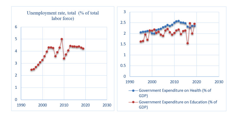
This study looks at how Bangladesh's human capital investment has affected unemployment from 1995 to 2019. To identify the study's unit root, we employed the ADF and PP tests. The short- term and long-term impacts of human capital investment on unemployment are estimated using the Autoregressive Distributive Lag (ARDL) model. The presence or absence of cointegration is assessed using the ARDL bound cointegration test. The Pairwise Granger Causality test, in contrast, is used to ascertain whether there exist causal relationships between variables. The study's findings demonstrate that government health spending on human capital has a significant impact on Bangladesh's long-term unemployment rate. Government spending on education and the unemployment rate are causally related in a single direction, according to the Pairwise Granger test. In the short term, the analysis showed no discernible relationship between human capital investment and unemployment rates. To build a healthy nation and eventually lower Bangladesh's unemployment rate, it is urged that the government should increase health spending and strengthen the health sector. To connect education with employment, the government may give vocational and career-focused education equal weight with general education.
Citation: Mahinur Begum Mimi, Md. Ahasan Ul Haque, Md. Golam Kibria. Does human capital investment influence unemployment rate in Bangladesh: a fresh analysis[J]. National Accounting Review, 2022, 4(3): 273-286. doi: 10.3934/NAR.2022016
This study looks at how Bangladesh's human capital investment has affected unemployment from 1995 to 2019. To identify the study's unit root, we employed the ADF and PP tests. The short- term and long-term impacts of human capital investment on unemployment are estimated using the Autoregressive Distributive Lag (ARDL) model. The presence or absence of cointegration is assessed using the ARDL bound cointegration test. The Pairwise Granger Causality test, in contrast, is used to ascertain whether there exist causal relationships between variables. The study's findings demonstrate that government health spending on human capital has a significant impact on Bangladesh's long-term unemployment rate. Government spending on education and the unemployment rate are causally related in a single direction, according to the Pairwise Granger test. In the short term, the analysis showed no discernible relationship between human capital investment and unemployment rates. To build a healthy nation and eventually lower Bangladesh's unemployment rate, it is urged that the government should increase health spending and strengthen the health sector. To connect education with employment, the government may give vocational and career-focused education equal weight with general education.

| [1] | Bashir F, Farooq S, Nawaz S, et al. (2012) Education, health and employment in Pakistan: a co-integration analysis. Res Humanit Soc Sci 2: 53–64. |
| [2] | Becker, Gary S (1964) Human capital: a theoretical and empirical analysis, with special reference to education. New York: Columbia University Press. Available from: https://press.uchicago.edu/ucp/books/book/chicago/H/bo3684031.html. |
| [3] | Cazes S, Verick S (2013) Perspectives on labour economics for development. Geneva, Switzerland: International Labour Organization. Available from: https://www.ilo.org/global/publications/ilobookstore/orderonline/books/WCMS_190112/lang--en/index.htm. |
| [4] | Denny K, Harmon C (2000) The impact of education and training on the labour market experiences of young adults. IFS Working Papers. https://doi.org/10.1920/wp.ifs.2000.0008 |
| [5] |
Dickey DA, WA Fuller (1981) Likelihood Ratio Statistics for Autoregressive Time Series with a Unit Root. Econometrica 49: 1057–72. https://doi.org/10.2307/1912517 doi: 10.2307/1912517

|
| [6] | Faridi MZ, Malik S, Ahmad I (2010) Impact of education and health on employment in Pakistan: A case study. European Journal of Economics, Finance and Administrative Sciences. |
| [7] | Garrouste C, Kozovska K, Perez EA (2010) Education and long-term unemployment. Available from: https://hal.archives-ouvertes.fr/hal-03245305. |
| [8] |
Granger CW (1969) Investigating causal relations by econometric models and cross-spectral methods. Econometrica 37: 424–438. https://doi.org/10.2307/1912791 doi: 10.2307/1912791
|
| [9] | Huq MN, Howlader SR, Kabir MA (2014) The impact of health on productivity in Bangladesh. Global J Quant Sci 1: 24–31. |
| [10] | Kalwij A, Vermeulen F (2005) Labor force participation of the elderly in Europe: The importance of being healthy. http://dx.doi.org/10.2139/ssrn.875383 |
| [11] | Ke XU, Saksena P, Holly A (2011) The determinants of health expenditure: a country-level panel data analysis. Geneva: World Health Organization 26: 1–28. |
| [12] | Kenny SV (2019) Effects of Human Capital Investment on Unemployment Volatility in Nigeria. Available from: https://mpra.ub.unimuenchen.de/93295/1/MPRA_paper_93295.pdf. |
| [13] | Laplagne P, Glover M, Shomos A (2007) Effects of health and education on labor force participation. http://dx.doi.org/10.2139/ssrn.1018889 |
| [14] | Lewis WA (1954) Economic development with unlimited supplies of labor. Available from: http://la.utexas.edu/users/hcleaver/368/368lewistable.pdf. |
| [15] | Mete C, Schultz TP (2002) Health and labor force participation of the elderly in Taiwan. Available from: https://ssrn.com/abstract=317981. |
| [16] | Mincer J (1958) Investment in human capital and personal income distribution. J Polit Econ 66: 281–302. |
| [17] | Marshall A (1980) Principles of Economics. An Introductory Volume. London: Palgrave Macmillan. |
| [18] |
O'Higgins N, Ivanov A (2006) Education and employment opportunities for the Roma. Comp Econ Stud 48: 6–19. https://doi.org/10.1057/palgrave.ces.8100147 doi: 10.1057/palgrave.ces.8100147
|
| [19] | Okun AM (1962) Potential GNP & Its Measurement and Significance. Proceedings of the Business and Economics section, 98–104. |
| [20] |
Pelkowski JM, Berger MC (2004) The impact of health on employment, wages, and hours worked over the life cycle. Q Rev Econ Financ 44: 102–121. https://doi.org/10.1016/j.qref.2003.08.002 doi: 10.1016/j.qref.2003.08.002
|
| [21] |
Pesaran MH, Shin Y, Smith RJ (2001) Bounds testing approaches to the analysis of level of relationship. J Appl Economet 16: 289–326. https://doi.org/10.1002/jae.616 doi: 10.1002/jae.616
|
| [22] |
Philips PC, P Perron (1988) Testing for a Unit Root in Time Series Regression. Biometrika 75:335–46. https://doi.org/10.1093/biomet/75.2.335 doi: 10.1093/biomet/75.2.335
|
| [23] |
Phillips AW (1958) The relation between unemployment and the rate of change of money wage rates in the United Kingdom, 1861–1957. Economica 25: 283–299. https://doi.org/10.2307/2550759 doi: 10.2307/2550759
|
| [24] | Rahman M, Khan TI, Sabbih MA (2016) Budget for Education in Bangladesh An Analysis of Trends, Gaps and Priorities. Available from: https://www.campebd.org/Files/Budget%20for%20Education%20in%20Bangladesh-1.pdf. |
| [25] | Rahman RI (2006) Access to education and employment: Implications for poverty. Available from: https://socialprotection.gov.bd/wp-content/uploads/2017/06/Access-to-Education-and-Employment-Impact-on-Poverty.pdf. |
| [26] | Samiullah (2014) Relationship between Unemployment and Human Capital. J Resour Dev Manag 3: 1–11. |
| [27] | Schultz TW (1961) Investment in human capital. Am Econ Rev 51: 1–17. |
| [28] | Smith A (1776) An Inquiry into the Nature and Causes of the Wealth of Nations. Available from: https://ideas.repec.org/b/hay/hetboo/smith1776.html. |
| [29] | Statistics BBO (2011) Statistical yearbook of Bangladesh. Statistics Division, Ministry of Planning, Dhaka, Government of the People's Republic of Bangladesh. Available from: http://203.112.218.65:8008/WebTestApplication/userfiles/Image/LatestReports/YB2011.pdf. |
| [30] | Statistics BBO (2020) Statistical yearbook of Bangladesh. Statistics Division, Ministry of Planning, Dhaka, Government of the People's Republic of Bangladesh. Available from: http://www.bbs.gov.bd/site/page/29855dc1-f2b4-4dc0-9073f692361112da/Statistical-Yearbook. |
| [31] | Todaro MP, Smith SC (2011) Economic development (11th ed.). Boston, MA: Addison-Wesley. |
| [32] | World Bank (2021) World development indicators 2021. Available from: https://www.worldbank.org/en/publication/wdr2021. |
| [33] | Yusuf SM, Mogadishu S (2021) The Effect of Population Growth on Unemployment in Somalia. Available from: https://www.researchgate.net/publication/354555484. |
 NAR-04-03-016-s001.docx NAR-04-03-016-s001.docx |
 |
Figures(2) / Tables(5)

Mahinur Begum Mimi, Md. Ahasan Ul Haque, Md. Golam Kibria. Does human capital investment influence unemployment rate in Bangladesh: a fresh analysis[J]. National Accounting Review, 2022, 4(3): 273-286. doi: 10.3934/NAR.2022016


 DownLoad: