Dynamics and optimal control of a Zika model with sexual and vertical transmissions

Hai-Feng Huo; Tian Fu; Hong Xiang; Hai-Feng Huo; Tian Fu; Hong Xiang

doi:10.3934/mbe.2023361

Mathematical Biosciences and Engineering

2023, Volume 20, Issue 5: 8279-8304. doi: 10.3934/mbe.2023361

Previous Article Next Article

Research article

Dynamics and optimal control of a Zika model with sexual and vertical transmissions

Department of Applied Mathematics, Lanzhou University of Technology, Lanzhou, Gansu 730050, China

Academic Editor: Tonghua Zhang

Received: 27 November 2022 Revised: 08 February 2023 Accepted: 14 February 2023 Published: 28 February 2023

A new transmission model of Zika virus with three transmission routes including human transmission by mosquito bites, sexual transmission between males and females and vertical transmission is established. The basic reproduction number $ R_{0} $ is derived. When $ R_{0} < 1 $, it is proved that the disease-free equilibrium is globally stable. Furthermore, the optimal control and mitigation methods for transmission of Zika virus are deduced and explored. The MCMC method is used to estimate the parameters and the reasons for the deviation between the actual infection cases and the simulated data are discussed. In addition, different strategies for controlling the spread of Zika virus are simulated and studied. The combination of mosquito control strategies and internal human control strategies is the most effective way in reducing the risk of Zika virus infection.
- Zika virus,
- vertical transmission,
- sexual transmission,
- the basic reproduction number,
- optimal control
Citation: Hai-Feng Huo, Tian Fu, Hong Xiang. Dynamics and optimal control of a Zika model with sexual and vertical transmissions[J]. Mathematical Biosciences and Engineering, 2023, 20(5): 8279-8304. doi: 10.3934/mbe.2023361

Related Papers:

Abstract

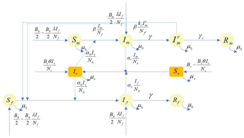
A new transmission model of Zika virus with three transmission routes including human transmission by mosquito bites, sexual transmission between males and females and vertical transmission is established. The basic reproduction number $ R_{0} $ is derived. When $ R_{0} < 1 $, it is proved that the disease-free equilibrium is globally stable. Furthermore, the optimal control and mitigation methods for transmission of Zika virus are deduced and explored. The MCMC method is used to estimate the parameters and the reasons for the deviation between the actual infection cases and the simulated data are discussed. In addition, different strategies for controlling the spread of Zika virus are simulated and studied. The combination of mosquito control strategies and internal human control strategies is the most effective way in reducing the risk of Zika virus infection.

References

[1]	G. W. Dick, S. F. Kitchen, A. J. Haddow, Zika virus (Ⅰ). Isolations and serological specificity, Trans. R. Soc. Trop. Med. Hyg., 46 (1952), 509–520. https://doi.org/10.1016/0035-9203(52)90042-4 doi: 10.1016/0035-9203(52)90042-4
[2]	L. R. Petersen, D. J. Jamieson, A. M. Powers, M. A. Honein, Zika virus, N. Engl. J. Med., 374 (2016), 1552–1563. https://doi.org/10.1056/nejmra1602113 doi: 10.1056/nejmra1602113
[3]	Centers for Disease Control and Prevention, About Zika, Overview, Available from: https://www.cdc.gov/zika/about/overview.html.
[4]	K. Smithburn, Neutralizing antibodies against certain recently isolated viruses in the sera of human beings residing in East Africa, J. Immunol., 69 (1952), 223–234. https://doi.org/10.4049/jimmunol.69.2.223 doi: 10.4049/jimmunol.69.2.223
[5]	M. R. Duffy, T. H. Chen, W. T. Hancock, A. M. Powers, J. L. Kool, R. S. Lanciotti, et al., Zika virus outbreak on Yap Island, federated states of Micronesia, N. Engl. J. Med., 360 (2009), 2536–2543. https://doi.org/10.1056/NEJMoa0805715 doi: 10.1056/NEJMoa0805715
[6]	D. Musso, E. Nilles, V. M. Cao Lormeau, Rapid spread of emerging Zika virus in the Pacific area, Clin. Microbiol. Infect., 20 (2014), O595–O596. https://doi.org/10.1111/1469-0691.12707 doi: 10.1111/1469-0691.12707
[7]	World Health Organization, Zika virus outbreak global response-Interim report May 2016. Available from: https://www.who.int/publications/i/item/zika-virus-outbreak-global-response.
[8]	J. Mlakar, M. Korva, N. Tul, M. Popović, M. Poljšak-Prijatelj, J. Mraz, et al., Zika virus associated with microcephaly, N. Engl. J. Med., 374 (2016), 951–958. https://doi.org/10.1056/NEJMoa1600651 doi: 10.1056/NEJMoa1600651
[9]	P. S. Mead, N. K. Duggal, S. A. Hook, M. Delorey, M. Fischer, D. O. McGuire, et al., Zika virus shedding in semen of symptomatic infected men N. Engl. J. Med., 378 (2018), 1377–1385. https://doi.org/10.1056/NEJMoa1711038 doi: 10.1056/NEJMoa1711038
[10]	Centers for Disease Control and Prevention, Questions About Zika, Available from: https://www.who.int/publications/i/item/zika-virus-outbreak-global-response.
[11]	B. D. Foy, K. C. Kobylinski, J. L. C. Foy, B. J. Blitvich, A. T. da Rosa, A. D. Haddow, et al., Probable non¨Cvector-borne transmission of Zika virus, Colorado, USA, Emerging Infect. Dis., 17 (2011), 880–882. https://doi.org/10.3201/eid1705.101939 doi: 10.3201/eid1705.101939
[12]	D. Gao, Y. Lou, D. He, T. C. Porco, Y. Kuang, G. Chowell, et al., Prevention and control of Zika as a mosquito-borne and sexually transmitted disease: a mathematical modeling analysis, Sci. Rep., 6 (2016), 1–10. https://doi.org/10.1038/srep28070 doi: 10.1038/srep28070
[13]	D. He, D. Gao, Y. Lou, S. Zhao, S. Ruan, A comparison study of Zika virus outbreaks in French Polynesia, Colombia and the State of Bahia in Brazil, Sci. Rep., 7 (2017), 273. https://doi.org/10.1038/s41598-017-00253-1 doi: 10.1038/s41598-017-00253-1
[14]	D. Baca-Carrasco, J. X. Velasco-Hernández, Sex, mosquitoes and epidemics: An evaluation of Zika disease dynamics, Bull. Math. Biol., 78 (2016), 2228–2242. https://doi.org/10.1007/s11538-016-0219-4 doi: 10.1007/s11538-016-0219-4
[15]	F. Agusto, S. Bewick, W. Fagan, Mathematical model for Zika virus dynamics with sexual transmission route, Ecol. Complex, 29 (2017), 61–81. https://doi.org/10.1016/j.ecocom.2016.12.007 doi: 10.1016/j.ecocom.2016.12.007
[16]	M. Imran, M. Usman, M. Dur-e Ahmad, A. Khan, Transmission dynamics of Zika fever: A SEIR based model, Differ. Equtions Dyn. Syst., 29 (2021), 463–486. https://doi.org/10.1007/s12591-017-0374-6 doi: 10.1007/s12591-017-0374-6
[17]	A. D¡äenes, M. A. Ibrahim, L. Oluoch, M. Tekeli, T. Tekeli, Impact of weather seasonality and sexual transmission on the spread of Zika fever, Sci. Rep., 9 (2019), 17055. https://doi.org/10.1038/s41598-019-53062-z doi: 10.1038/s41598-019-53062-z
[18]	M. A. Ibrahim, A. Dénes, Threshold dynamics in a model for Zika virus disease with seasonality, Bull. Math. Biol., 83 (2021), 27. https://doi.org/10.1007/s11538-020-00844-6 doi: 10.1007/s11538-020-00844-6
[19]	X. Yuan, Y. Lou, D. He, J. Wang, D. Gao, A Zika endemic model for the contribution of multiple transmission routes, Bull. Math. Biol., 83 (2021), 111. https://doi.org/10.1007/s11538-021-00945-w doi: 10.1007/s11538-021-00945-w
[20]	S. Busenberg, K. Cooke, Vertically Transmitted Diseases: Models and Dynamics, Biomathematics 23, Springer-Verlag, Berlin Heidelberg, 1993.
[21]	M. Y. Li, H. L. Smith, L. Wang, Global dynamics of an SEIR epidemic model with vertical transmission, SIAM J. Appl. Math., 62 (2001), 58–69. https://doi.org/10.1137/S0036139999359860 doi: 10.1137/S0036139999359860
[22]	S. Olaniyi, Dynamics of Zika virus model with nonlinear incidence and optimal control strategies, Appl. Math. Inf. Sci., 12 (2018), 969–982. https://doi.org/10.18576/amis/120510 doi: 10.18576/amis/120510
[23]	E. Okyere, S. Olaniyi, E. Bonyah, Analysis of zika virus dynamics with sexual transmission route using multiple optimal controls, Sci. Afr., 9 (2020), e00532. https://doi.org/10.1016/j.sciaf.2020.e00532 doi: 10.1016/j.sciaf.2020.e00532
[24]	P. Van den Driessche, J. Watmough, Reproduction numbers and sub-threshold endemic equilibria for compartmental models of disease transmission, Math. Biosci., 180 (2002), 29–48. https://doi.org/10.1016/S0025-5564(02)00108-6 doi: 10.1016/S0025-5564(02)00108-6
[25]	S. Wiggins, Introduction to Applied Nonlinear Dynamical Systems and Chaos, Springer, Berlin, 1990.
[26]	F. B. Agusto, S. Bewick, W. Fagan, Mathematical model of Zika virus with vertical transmission, Infect. Dis. Modell., 2 (2017), 244–267. https://doi.org/10.1016/j.idm.2017.05.003 doi: 10.1016/j.idm.2017.05.003
[27]	K. Blayneh, Y. Cao, H. D. Kwon, Optimal control of vector-borne diseases: Treatment and prevention, Discrete Contin. Dyn. Syst. Ser. B, 11 (2009), 587–611. https://doi.org/10.3934/DCDSB.2009.11.587 doi: 10.3934/DCDSB.2009.11.587
[28]	C. Castillo-Chavez, S. Blower, P. Van den Driessche, D. Kirschner, A. A. Yakubu, Mathematical Approaches for Emerging and Reemerging Infectious Diseases, Springer-Verlag, New York, 2002.
[29]	C. Bhunu, W. Garira, Z. Mukandavire, Modeling HIV/AIDS and tuberculosis coinfection, Bull. Math. Biol., 71 (2009), 1745–1780. https://doi.org/10.1007/s11538-009-9423-9 doi: 10.1007/s11538-009-9423-9
[30]	L. Pontryagin, V. Boltyanskiy, R. Gamkrelidze, E. Mishchenko, Mathematical Theory of Optimal Processes, Interscience, New York, 1962.
[31]	S. Abimbade, S. Olaniyi, O. Ajala, M. Ibrahim, Optimal control analysis of a tuberculosis model with exogenous re-infection and incomplete treatment, Optim. Control Appl. Methods, 41 (2020), 2349–2368. https://doi.org/10.1002/oca.2658 doi: 10.1002/oca.2658
[32]	S. Olaniyi, O. Falowo, K. Okosun, M. Mukamuri, O. Obabiyi, O. Adepoju, Effect of saturated treatment on malaria spread with optimal intervention, Alexandria Eng. J., 65 (2023), 443–459. https://doi.org/10.1016/j.aej.2022.09.024 doi: 10.1016/j.aej.2022.09.024
[33]	D. L. Lukes, Differential Equations: Classical to Controlled, Academic Press, 162 (1982), 223–225. https://doi.org/10.2307/2322889
[34]	A. Abidemi, S. Olaniyi, O. A. Adepoju, An explicit note on the existence theorem of optimal control problem, J. Phys. Conf. Ser., 2199 (2022), 012021. https://doi.org/10.1088/1742-6596/2199/1/012021 doi: 10.1088/1742-6596/2199/1/012021
[35]	World Health Organization, WHO Global Health Observatory data repository, Crude birth and death rate. Data by country, 2003. Available from: https://apps.who.int/gho/data/node.main.CBDR107?lang = en.
[36]	A. C. Gourinat, O. OConnor, E. Calvez, C. Goarant, M. Dupont-Rouzeyrol, Detection of Zika virus in urine, Emerging Infect. Dis., 21 (2015), 84–86. https://doi.org/10.3201/eid2101.140894 doi: 10.3201/eid2101.140894
[37]	D. Musso, C. Roche, E. Robin, T. Nhan, A. Teissier, V. M. Cao-Lormeau, Potential sexual transmission of Zika virus, Emerging Infect. Dis., 21 (2015), 359–361. https://doi.org/10.3201/eid2102.141363 doi: 10.3201/eid2102.141363

Reader Comments

Your name:*

Email:*
© 2023 the Author(s), licensee AIMS Press. This is an open access article distributed under the terms of the Creative Commons Attribution License (http://creativecommons.org/licenses/by/4.0)