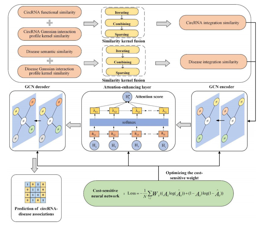
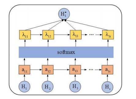
Circular RNAs (circRNAs) constitute a category of circular non-coding RNA molecules whose abnormal expression is closely associated with the development of diseases. As biological data become abundant, a lot of computational prediction models have been used for circRNA–disease association prediction. However, existing prediction models ignore the non-linear information of circRNAs and diseases when fusing multi-source similarities. In addition, these models fail to take full advantage of the vital feature information of high-similarity neighbor nodes when extracting features of circRNAs or diseases. In this paper, we propose a deep learning model, CDA-SKAG, which introduces a similarity kernel fusion algorithm to integrate multi-source similarity matrices to capture the non-linear information of circRNAs or diseases, and construct a circRNA information space and a disease information space. The model embeds an attention-enhancing layer in the graph autoencoder to enhance the associations between nodes with higher similarity. A cost-sensitive neural network is introduced to address the problem of positive and negative sample imbalance, consequently improving our model's generalization capability. The experimental results show that the prediction performance of our model CDA-SKAG outperformed existing circRNA–disease association prediction models. The results of the case studies on lung and cervical cancer suggest that CDA-SKAG can be utilized as an effective tool to assist in predicting circRNA–disease associations.
Citation: Huiqing Wang, Jiale Han, Haolin Li, Liguo Duan, Zhihao Liu, Hao Cheng. CDA-SKAG: Predicting circRNA-disease associations using similarity kernel fusion and an attention-enhancing graph autoencoder[J]. Mathematical Biosciences and Engineering, 2023, 20(5): 7957-7980. doi: 10.3934/mbe.2023345
Circular RNAs (circRNAs) constitute a category of circular non-coding RNA molecules whose abnormal expression is closely associated with the development of diseases. As biological data become abundant, a lot of computational prediction models have been used for circRNA–disease association prediction. However, existing prediction models ignore the non-linear information of circRNAs and diseases when fusing multi-source similarities. In addition, these models fail to take full advantage of the vital feature information of high-similarity neighbor nodes when extracting features of circRNAs or diseases. In this paper, we propose a deep learning model, CDA-SKAG, which introduces a similarity kernel fusion algorithm to integrate multi-source similarity matrices to capture the non-linear information of circRNAs or diseases, and construct a circRNA information space and a disease information space. The model embeds an attention-enhancing layer in the graph autoencoder to enhance the associations between nodes with higher similarity. A cost-sensitive neural network is introduced to address the problem of positive and negative sample imbalance, consequently improving our model's generalization capability. The experimental results show that the prediction performance of our model CDA-SKAG outperformed existing circRNA–disease association prediction models. The results of the case studies on lung and cervical cancer suggest that CDA-SKAG can be utilized as an effective tool to assist in predicting circRNA–disease associations.

| [1] |
W. R. Jeck, N. E. Sharpless, Detecting and characterizing circular RNAs, Nat. Biotechnol., 32 (2014), 453–461. https://doi.org/10.1038/nbt.2890 doi: 10.1038/nbt.2890

|
| [2] |
L. Salmena, L. Poliseno, Y. Tay, L. Kats, P. Pandolfi, A ceRNA hypothesis: the Rosetta Stone of a hidden RNA language, Cell, 146 (2011), 353–358. https://doi.org/10.1016/j.cell.2011.07.014 doi: 10.1016/j.cell.2011.07.014
|
| [3] |
Y. Zhang, X. Zhang, T. Chen, J. Xiang, Q. Yin, Y. Xing, Circular intronic long noncoding RNAs, Mol. Cell, 51 (2013), 792–806. https://doi.org/10.1016/j.molcel.2013.08.017 doi: 10.1016/j.molcel.2013.08.017
|
| [4] |
C. Wang, C. Han, Q. Zhao, X. Chen, Circular RNAs and complex diseases: from experimental results to computational models, Brief. Bioinform., 22 (2021), 1–27. https://doi.org/10.1093/bib/bbab286 doi: 10.1093/bib/bbab286
|
| [5] |
V. M. Conn, V. Hugouvieux, A. Nayak, S. A. Conos, G. Capovilla, G. Cildir, A circRNA from SEPALLATA3 regulates splicing of its cognate mRNA through R-loop formation, Nat. Plants, 3 (2017), 1–5. https://doi.org/10.1038/nplants.2017.53 doi: 10.1038/nplants.2017.53
|
| [6] |
G. Liang, Y. Ling, M. Mehrpour, P. E. Saw, Z. Liu, W. Tan, Autophagy-associated circRNA circCDYL augments autophagy and promotes breast cancer progression, Mol Cancer, 19 (2020), 1–16. https://doi.org/10.1186/s12943-020-01152-2 doi: 10.1186/s12943-020-01152-2
|
| [7] |
S. Zhang, X. Chen, C. Li, X. Li, Identification and characterization of circular RNAs as a new class of putative biomarkers in diabetes retinopathy, Invest. Ophthalmol. Vis. Sci., 58 (2017), 6500–6509. https://doi.org/10.1167/iovs.17-22698 doi: 10.1167/iovs.17-22698
|
| [8] |
C. Ma, X. Wang, F. Yang, Y. Zang, J. Liu, X. Wang, Circular RNA hsa_circ_0004872 inhibits gastric cancer progression via the miR-224/Smad4/ADAR1 successive regulatory circuit, Mol. Cancer, 19 (2020), 1–21. https://doi.org/10.1186/s12943-020-01268-5 doi: 10.1186/s12943-020-01268-5
|
| [9] |
M. Jamal, T. Song, B. Chen, M. Faisal, Z. Hong, T. Xie, Recent progress on circular RNA research in acute myeloid leukemia, Front. Oncol., 9 (2019), 1–13. https://doi.org/10.3389/fonc.2019.01108 doi: 10.3389/fonc.2019.01108
|
| [10] |
J. Zhang, H. Sun, Roles of circular RNAs in diabetic complications: From molecular mechanisms to therapeutic potential, Gene, 763 (2020), 1–11. https://doi.org/10.1016/j.gene.2020.145066 doi: 10.1016/j.gene.2020.145066
|
| [11] |
Z. Mohamed, circRNAs signature as potential diagnostic and prognostic biomarker for diabetes mellitus and related cardiovascular complications, Cells, 9 (2020), 1–19. https://doi.org/10.3390/cells9030659 doi: 10.3390/cells9030659
|
| [12] |
Y. Zhou, J. Hu, Z. Shen, W. Zhang, P. Du, LPI-SKF: predicting lncRNA-protein interactions using similarity kernel fusions, Front. Genet., 11 (2020), 1–11. https://doi.org/10.3389/fgene.2020.615144 doi: 10.3389/fgene.2020.615144
|
| [13] |
K. Deepthi, A. S. Jereesh, Inferring potential CircRNA–disease associations via deep autoencoder-based classification, Mol. Diagn. Ther, 25 (2021), 87–97. https://doi.org/10.1007/s40291-020-00499-y doi: 10.1007/s40291-020-00499-y
|
| [14] |
K. Deepthi, A. S. Jereesh, An ensemble approach for circRNA–disease association prediction based on autoencoder and deep neural network, Gene, 762 (2020), 1–7. https://doi.org/10.1016/j.gene.2020.145040 doi: 10.1016/j.gene.2020.145040
|
| [15] |
Z. Ma, Z. Kuang, L. Deng, CRPGCN: predicting circRNA–disease associations using graph convolutional network based on heterogeneous network, BMC Bioinform., 22 (2021), 1–23. https://doi.org/10.1186/s12859-021-04467-z doi: 10.1186/s12859-021-04467-z
|
| [16] |
C. Shi, B. Hu, W. Zhao, P. Yu, Heterogeneous information network embedding for recommendation, IEEE Trans. Knowl. Data Eng., 31 (2018), 357–370. https://doi.org/10.1109/TKDE.2018.2833443 doi: 10.1109/TKDE.2018.2833443
|
| [17] |
K. Zheng, Z. You, J. Li, L. Wang, Z. Guo, Y. Huang, iCDA-CGR: Identification of circRNA–disease associations based on chaos game representation, PLoS Comput. Biol., 16 (2020), 1–22. https://doi.org/10.1371/journal.pcbi.1007872 doi: 10.1371/journal.pcbi.1007872
|
| [18] |
L. Jiang, Y. Ding, J. Tang, F. Guo, MDA-SKF: similarity kernel fusion for accurately discovering miRNA-disease association, Front. Genet., 9 (2018), 1–13. https://doi.org/10.3389/fgene.2018.00618 doi: 10.3389/fgene.2018.00618
|
| [19] |
G. Li, Y. Lin, J. Luo, Q. Xiao, C. Liang, GGAECDA: Predicting circRNA–disease associations using graph autoencoder based on graph representation learning, Comput. Biol. Chem., 99 (2022), 1–10. https://doi.org/10.1016/j.compbiolchem.2022.107722 doi: 10.1016/j.compbiolchem.2022.107722
|
| [20] |
X. Wu, W. Lan, Q. Chen, Y. Dong, J. Liu, W. Peng, Inferring LncRNA-disease associations based on graph autoencoder matrix completion, Comput. Biol. Chem., 87 (2020), 1–7. https://doi.org/10.1016/j.compbiolchem.2020.107282 doi: 10.1016/j.compbiolchem.2020.107282
|
| [21] | T. N. Kipf, M. Welling, Variational graph auto-encoders, arXiv e-prints, 2016, 1–3. https://arXiv.org/abs/1611.07308 |
| [22] |
W. Wang, L. Zhang, J. Sun, Q. Zhao, J. Shuai, Predicting the potential human lncRNA–miRNA interactions based on graph convolution network with conditional random field, Brief. Bioinform., 23 (2022), 1–9. https://doi.org/10.1093/bib/bbac463 doi: 10.1093/bib/bbac463
|
| [23] | L. Wang, Z. You, D. Huang, J. Li, MGRCDA: Metagraph recommendation method for predicting circRNA–disease association, in IEEE Transactions on Cybernetics, 53 (2023), 67–75. https://doi.org/10.1109/TCYB.2021.3090756 |
| [24] | B. Kang, S. Xie, M. Rohrbach, Z. Yan, A. Gordo, Decoupling representation and classifier for long-tailed recognition, in International Conference on Learning Representations, (2019), 1–14. https://arXiv.org/abs/1910.09217 |
| [25] |
H. Guo, Y. Li, J. Shang, M. Gu, Y. Huang, B. Gong, Learning from class-imbalanced data: Review of methods and applications, Expert Syst. Appl., 73 (2017), 220–239. https://doi.org/10.1016/j.eswa.2016.12.035 doi: 10.1016/j.eswa.2016.12.035
|
| [26] |
X. Zeng, Y. Zhong, W. Lin, Q. Zou, Predicting disease-associated circular RNAs using deep forests combined with positive-unlabeled learning methods, Brief. Bioinform., 21 (2020), 1425–1436. https://doi.org/10.1093/bib/bbz080 doi: 10.1093/bib/bbz080
|
| [27] |
P. Yang, X. Li, J. Mei, C. Kwoh, S. Ng, Positive-unlabeled learning for disease gene identification, Bioinformatics, 28 (2012), 2640–2647. https://doi.org/10.1093/bioinformatics/bts504 doi: 10.1093/bioinformatics/bts504
|
| [28] |
Z. Cheng, S. Zhou, Y. Wang, H. Liu, J. Guan, Effectively identifying compound-protein interactions by learning from positive and unlabeled examples, IEEE/ACM Trans Comput. Biol. Bioinform., 15 (2016), 1832–1843. https://doi.org/10.1109/TCBB.2016.2570211 doi: 10.1109/TCBB.2016.2570211
|
| [29] |
L. Wang, L. Wong, Z. Li, Y. Huang, X. Su, B. Zhao, Z. You, A machine learning framework based on multi-source feature fusion for circRNA–disease association prediction, Brief. Bioinform., 23 (2022), 1–9. https://doi.org/10.1093/bib/bbac388 doi: 10.1093/bib/bbac388
|
| [30] | C. Wan, L. Wang, K. Ting, Introducing cost-sensitive neural networks, in Processing of The Second International Conference on information, Communications, and Signal Processing (ICICS 99), (1999), 1–4. |
| [31] |
C. Fan, X. Lei, Z. Fang, Q. Jiang, F. Wu, CircR2Disease: a manually curated database for experimentally supported circular RNAs associated with various diseases, Database, 2018 (2018), 1–6. https://doi.org/10.1093/database/bay044 doi: 10.1093/database/bay044
|
| [32] |
L. M. Schriml, C. Arze, S. Nadendla, Y. Chang, M. Mazaitis, V. Felix, et al., Disease ontology: a backbone for disease semantic integration, Nucleic Acids Res., 40 (2012), 940–946. https://doi.org/10.1093/nar/gkr972 doi: 10.1093/nar/gkr972
|
| [33] |
G. Yu, L. Wang, G. Yan, Q. He, DOSE: an R/Bioconductor package for disease ontology semantic and enrichment analysis, Bioinformatics, 31 (2015), 608–609. https://doi.org/10.1093/bioinformatics/btu684 doi: 10.1093/bioinformatics/btu684
|
| [34] |
D. Wang, J. Wang, M. Lu, F. Song, Q. Cui, Inferring the human microRNA functional similarity and functional network based on microRNA-associated diseases, Bioinformatics, 26 (2010), 1644–1650. https://doi.org/10.1093/bioinformatics/btq241 doi: 10.1093/bioinformatics/btq241
|
| [35] |
T. V. Laarhoven, S. B. Nabuurs, E. Marchiori, Gaussian interaction profile kernels for predicting drug–target interaction, Bioinformatics, 27 (2011), 3036–3043. https://doi.org/10.1093/bioinformatics/btr500 doi: 10.1093/bioinformatics/btr500
|
| [36] | D. Bahdanau, K. Cho, Y. Bengio, Neural machine translation by jointly learning to align and translate, in International Conference on Learning Representations, (2015), 1–15. https://arXiv.org/abs/1409.0473 |
| [37] | H. Gao, J. Pei, H. Huang, Conditional random field enhanced graph convolutional neural networks, in Proceedings of the 25th ACM SIGKDD International Conference on Knowledge Discovery & Data Mining, (2019), 276–284. https://doi.org/10.1145/3292500.3330888 |
| [38] |
Y. Long, M. Wu, C. K. Kwoh, J. Luo, X. Li, Predicting human microbe–drug associations via graph convolutional network with conditional random field, Bioinformatics, 36 (2020), 4918–4927. https://doi.org/10.1093/bioinformatics/btaa598 doi: 10.1093/bioinformatics/btaa598
|
| [39] | D. P. Kingma, J. Ba, Adam: A method for stochastic optimization, in International Conference on Learning Representations, (2014), 1–15. https://arXiv.org/abs/1412.6980 |
| [40] |
C. Fan, X. Lei, Y. Pan, Prioritizing CircRNA–disease associations with convolutional neural network based on multiple similarity feature fusion, Front. Genet., 11 (2020), 1–13. https://doi.org/10.3389/fgene.2020.540751 doi: 10.3389/fgene.2020.540751
|
| [41] | Q. Li, Z. Han, X. Wu, Deeper insights into graph convolutional networks for semi-supervised learning, Proceed. AAAI, 32 (2018), 3538–3545. https://arXiv.org/abs/1801.07606 |
| [42] |
D. Chen, Y. Lin, W. Li, P. Li, J. Zhou, X. Sun, Measuring and relieving the over-smoothing problem for graph neural networks from the topological view, Proceed. AAAI Conf. Artif. Intell., 34 (2020), 3438–3445. https://doi.org/10.1609/aaai.v34i04.5747 doi: 10.1609/aaai.v34i04.5747
|
| [43] |
Z. Zuo, R. Cao, P. Wei, J. Xia, C. Zheng, Double matrix completion for circRNA–disease association prediction, BMC Bioinform., 22 (2021), 1–15. https://doi.org/10.1186/s12859-021-04231-3 doi: 10.1186/s12859-021-04231-3
|
| [44] |
C. Lu, M. Zeng, F. Zhang, F. Wu, M. Li, J. Wang, Deep matrix factorization improves prediction of human circRNA–disease associations, IEEE J. Biomed. Health Inform., 25 (2020), 891–899. https://doi.org/10.1109/JBHI.2020.2999638 doi: 10.1109/JBHI.2020.2999638
|
| [45] |
M. Niu, Q. Zou, C. Wang, GMNN2CD: identification of circRNA–disease associations based on variational inference and graph Markov neural networks, Bioinformatics, 38 (2022), 2246–2253. https://doi.org/10.1093/bioinformatics/btac079 doi: 10.1093/bioinformatics/btac079
|
| [46] |
E. Ge, Y. Yang, M. Gang, C. Fan, Q. Zhao, Predicting human disease-associated circRNAs based on locality-constrained linear coding, Genomics, 112 (2020), 1335–1342. https://doi.org/10.1016/j.ygeno.2019.08.001 doi: 10.1016/j.ygeno.2019.08.001
|
| [47] |
Z. Zhao, K. Wang, F. Wu, W. Wang, K. Zhang, H. Hu, circRNA disease: a manually curated database of experimentally supported circRNA–disease associations, Cell Death Dis., 9 (2018), 1–2. https://doi.org/10.1038/s41419-018-0503-3 doi: 10.1038/s41419-018-0503-3
|
| [48] |
Q. Zhao, Y. Yang, G. Ren, E. Ge, C. Fan, Integrating bipartite network projection and KATZ measure to identify novel circRNA–disease associations, IEEE Trans. Nanobiosci., 18 (2019), 578–584. https://doi.org/10.1109/TNB.2019.2922214 doi: 10.1109/TNB.2019.2922214
|
| [49] |
L. Zhang, P. Yang, H. Feng, Q. Zhao, H. Liu, Using network distance analysis to predict lncRNA–miRNA interactions, Interdiscip. Sci. Comput. Life Sci., 13 (2021), 535–545. https://doi.org/10.1007/s12539-021-00458-z doi: 10.1007/s12539-021-00458-z
|
| [50] |
F. Sun, J. Sun, Q. Zhao, A deep learning method for predicting metabolite–disease associations via graph neural network, Brief. Bioinform., 23 (2022), 1–11. https://doi.org/10.1093/bib/bbac266 doi: 10.1093/bib/bbac266
|
| [51] |
L. Guo, Z. You, L. Wang, C. Yu, B. Zhao, Z. Ren, et al., A novel circRNA-miRNA association prediction model based on structural deep neural network embedding, Brief. Bioinform., 23 (2022), 1–10. https://doi.org/10.1093/bib/bbac391 doi: 10.1093/bib/bbac391
|
Figures(7) / Tables(7)

Huiqing Wang, Jiale Han, Haolin Li, Liguo Duan, Zhihao Liu, Hao Cheng. CDA-SKAG: Predicting circRNA-disease associations using similarity kernel fusion and an attention-enhancing graph autoencoder[J]. Mathematical Biosciences and Engineering, 2023, 20(5): 7957-7980. doi: 10.3934/mbe.2023345


 DownLoad: