A full-flow inspection method based on machine vision to detect wafer surface defects

Naigong Yu; Hongzheng Li; Qiao Xu; Naigong Yu; Hongzheng Li; Qiao Xu

doi:10.3934/mbe.2023526

Mathematical Biosciences and Engineering

2023, Volume 20, Issue 7: 11821-11846. doi: 10.3934/mbe.2023526

Previous Article Next Article

Research article Special Issues

A full-flow inspection method based on machine vision to detect wafer surface defects

1.
Faculty of Information Technology, Beijing University of Technology, Beijing 100124, China
2.
Beijing Key Laboratory of Computing Intelligence and Intelligent System, Beijing University of Technology, Beijing 100124, China
3.
Engineering Research Center of Digital Community, Ministry of Education, Beijing 100124, China

Academic Editor: Chunwei Tian

Received: 13 March 2023 Revised: 24 April 2023 Accepted: 27 April 2023 Published: 09 May 2023

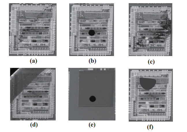
The semiconductor manufacturing industry relies heavily on wafer surface defect detection for yield enhancement. Machine learning and digital image processing technologies have been used in the development of various detection algorithms. However, most wafer surface inspection algorithms are not be applied in industrial environments due to the difficulty in obtaining training samples, high computational requirements, and poor generalization. In order to overcome these difficulties, this paper introduces a full-flow inspection method based on machine vision to detect wafer surface defects. Starting with the die image segmentation stage, where a die segmentation algorithm based on candidate frame fitting and coordinate interpolation is proposed for die sample missing matching segmentation. The method can segment all the dies in the wafer, avoiding the problem of missing dies splitting. After that, in the defect detection stage, we propose a die defect anomaly detection method based on defect feature clustering by region, which can reduce the impact of noise in other regions when extracting defect features in a single region. The experiments show that the proposed inspection method can precisely position and segment die images, and find defective dies with an accuracy of more than 97%. The defect detection method proposed in this paper can be applied to inspect wafer manufacturing.
- machine vision,
- wafer surface defect detection,
- machine learning,
- image segmentation,
- feature extraction
Citation: Naigong Yu, Hongzheng Li, Qiao Xu. A full-flow inspection method based on machine vision to detect wafer surface defects[J]. Mathematical Biosciences and Engineering, 2023, 20(7): 11821-11846. doi: 10.3934/mbe.2023526

Related Papers:

Abstract

The semiconductor manufacturing industry relies heavily on wafer surface defect detection for yield enhancement. Machine learning and digital image processing technologies have been used in the development of various detection algorithms. However, most wafer surface inspection algorithms are not be applied in industrial environments due to the difficulty in obtaining training samples, high computational requirements, and poor generalization. In order to overcome these difficulties, this paper introduces a full-flow inspection method based on machine vision to detect wafer surface defects. Starting with the die image segmentation stage, where a die segmentation algorithm based on candidate frame fitting and coordinate interpolation is proposed for die sample missing matching segmentation. The method can segment all the dies in the wafer, avoiding the problem of missing dies splitting. After that, in the defect detection stage, we propose a die defect anomaly detection method based on defect feature clustering by region, which can reduce the impact of noise in other regions when extracting defect features in a single region. The experiments show that the proposed inspection method can precisely position and segment die images, and find defective dies with an accuracy of more than 97%. The defect detection method proposed in this paper can be applied to inspect wafer manufacturing.

References

[1]	N. Yu, Q. Xu, H. Wang, J. Lin, Wafer bin map inspection based on densenet, J. Cent. South Univ., 28 (2021), 2436–2450. https://doi.org/10.1007/s11771-021-4778-7 doi: 10.1007/s11771-021-4778-7
[2]	L. Alam, N. Kehtarnavaz, A survey of detection methods for die attachment and wire bonding defects in integrated circuit manufacturing, IEEE Access, 10 (2022), 83826–83840. https://doi.org/10.1109/ACCESS.2022.3197624 doi: 10.1109/ACCESS.2022.3197624
[3]	Y. Fu, X. Ma, H. Zhou, Automatic detection of multi-crossing crack defects in multi-crystalline solar cells based on machine vision, Mach. Vision Appl., 32 (2021), 1–14. https://doi.org/10.1007/s00138-021-01183-9 doi: 10.1007/s00138-021-01183-9
[4]	Q. Hu, K. Hao, B. Wei, H. Li, An efficient solder joint defects method for 3d point clouds with double-flow region attention network, Adv. Eng. Inform., 52 (2022), 101608. https://doi.org/10.1016/j.aei.2022.101608 doi: 10.1016/j.aei.2022.101608
[5]	W. Dai, A. Mujeeb, M. Erdt, A. Sourin, Soldering defect detection in automatic optical inspection, Adv. Eng. Inform., 43 (2022), 101004. https://doi.org/10.1016/j.aei.2019.101004 doi: 10.1016/j.aei.2019.101004
[6]	T. Kim, K. Behdinan, Advances in machine learning and deep learning applications towards wafer map defect recognition and classification: a review, J. Intell. Manuf., (2022), 1–33. https://doi.org/10.1007/s10845-022-01994-1 doi: 10.1007/s10845-022-01994-1
[7]	K. C. Cheng, L. L. Chen, J. Li, K. S. Li, N. C. Tsai, S. Wang, et al., Machine learning-based detection method for wafer test induced defects, IEEE Trans. Semicond. Manuf., 34 (2021), 161–167. https://doi.org/10.1109/TSM.2021.3065405 doi: 10.1109/TSM.2021.3065405
[8]	J. Wang, Z. Yu, Z. Duan, G. Lu, A sub-region one-to-one mapping (som) detection algorithm for glass passivation parts wafer surface low-contrast texture defects, Multimedia Tools Appl., 80 (2021), 28879–28896. https://doi.org/10.1007/s11042-021-11084-8 doi: 10.1007/s11042-021-11084-8
[9]	K. S. Li, P. Y. Liao, K. C. Cheng, L. L. Chen, S. Wang, A. Y. Huang, et al., Hidden wafer scratch defects projection for diagnosis and quality enhancement, IEEE Trans. Semicond. Manuf., 34 (2020), 9–16. https://doi.org/10.1109/TSM.2020.3040998 doi: 10.1109/TSM.2020.3040998
[10]	N. Shankar, Z. Zhong, Defect detection on semiconductor wafer surfaces, Microelectron. Eng., 77 (2005), 337–346. https://doi.org/10.1016/j.mee.2004.12.003 doi: 10.1016/j.mee.2004.12.003
[11]	C. Yeh, F. Wu, W. Ji, C. Huang, A wavelet-based approach in detecting visual defects on semiconductor wafer dies, IEEE Trans. Semicond. Manuf., 23 (2010), 284–292. https://doi.org/10.1109/TSM.2010.2046108 doi: 10.1109/TSM.2010.2046108
[12]	Y. Chiou, J. Liu, Y. Liang, Micro crack detection of multi-crystalline silicon solar wafer using machine vision techniques, Sensor Rev., 31 (2011), 154–165. https://doi.org/10.1108/02602281111110013 doi: 10.1108/02602281111110013
[13]	M. Yao, J. Li, X. Wang, Solar cells surface defects detection using rpca method, Chin. J. Comput., 36 (2013), 1943–1952. https://doi.org/10.3724/SP.J.1016.2013.01943 doi: 10.3724/SP.J.1016.2013.01943
[14]	H. Lin, S. Chiu, Flaw detection of domed surfaces in led packages by machine vision system, Expert Syst. Appl., 38 (2011), 15208–15216. https://doi.org/10.1016/j.eswa.2011.05.080 doi: 10.1016/j.eswa.2011.05.080
[15]	Z. Zhang, Y. Liu, X. Wu, S. Kan, Integrated color defect detection method for polysilicon wafers using machine vision, Adv. Manuf., 2 (2014), 318–326. https://doi.org/10.1007/S40436-014-0095-9 doi: 10.1007/S40436-014-0095-9
[16]	N. Saad, A. Ahmad, H. Saleh, A. Hasan, Automatic semiconductor wafer image segmentation for defect detection using multilevel thresholding, in MATEC Web of Conferences, EDP Sciences, 2016. https://doi.org/10.1051/matecconf/20167801103
[17]	J. Ko, J. Rheem, Defect detection of polycrystalline solar wafers using local binary mean, Int. J. Adv. Manuf. Technol., 82 (2016), 1753–1764. https://doi.org/10.1007/s00170-015-7498-z doi: 10.1007/s00170-015-7498-z
[18]	Z. Wang, X. Liu, Z. He, L. Su, X. Lu, Intelligent detection of flip chip with the scanning acoustic microscopy and the general regression neural network, Microelectron. Eng., 217 (2019), 111127. https://doi.org/10.1016/j.mee.2019.111127 doi: 10.1016/j.mee.2019.111127
[19]	X. Chen, C. Zhao, J. Chen, D. Zhang, K. Zhu, Y. Su, K-means clustering with morphological filtering for silicon wafer grain defect detection, in 2020 IEEE 4th Information Technology, Networking, Electronic and Automation Control Conference (ITNEC), 1 (2020), 1251–1255. https://doi.org/10.1109/ITNEC48623.2020.9084726
[20]	B. M. Haddad, S. F. Dodge, L. J. Karam, N. S. Patel, M. W. Braun, Locally adaptive statistical background modeling with deep learning-based false positive rejection for defect detection in semiconductor units, IEEE Trans. Semicond. Manuf., 33 (2020), 357–372. https://doi.org/10.1109/TSM.2020.2998441 doi: 10.1109/TSM.2020.2998441
[21]	Y. Yang, M. Sun, Semiconductor defect detection by hybrid classical-quantum deep learning, in Proceedings of the IEEE/CVF Conference on Computer Vision and Pattern Recognition, (2022), 2323–2332. https://doi.org/10.1109/CVPR52688.2022.00236
[22]	H. Chen, Automated detection and classification of defective and abnormal dies in wafer images, Appl. Sci., 10 (2020), 3423. https://doi.org/10.3390/app10103423 doi: 10.3390/app10103423
[23]	J. O'Leary, K. Sawlani, A. Mesbah, Deep learning for classification of the chemical composition of particle defects on semiconductor wafers, IEEE Trans. Semicond. Manuf., 33 (2020), 72–85. https://doi.org/10.1109/TSM.2019.2963656 doi: 10.1109/TSM.2019.2963656
[24]	N. Yu, Q. Xu, H. Wang, Wafer defect pattern recognition and analysis based on convolutional neural network, IEEE Trans. Semicond. Manuf., 32 (2019), 566–573. https://doi.org/10.1109/TSM.2019.2937793 doi: 10.1109/TSM.2019.2937793
[25]	P. P. Shinde, P. P. Pai, S. P. Adiga, Wafer defect localization and classification using deep learning techniques, IEEE Access, 10 (2022), 39969–39974. https://doi.org/10.1109/ACCESS.2022.3166512 doi: 10.1109/ACCESS.2022.3166512
[26]	S. Chen, C. Kang, D. Perng, Detecting and measuring defects in wafer die using gan and yolov3, Appl. Sci., 10 (2020), 8725. https://doi.org/10.3390/app10238725 doi: 10.3390/app10238725
[27]	Y. Yi, S. Lai, W. Wang, S. Li, R. Zhang, Y. Luo, et al., Sdnmf: Semisupervised discriminative nonnegative matrix factorization for feature learning, Int. J. Intell. Syst., 37 (2022), 11547–11581. https://doi.org/10.1002/int.23054 doi: 10.1002/int.23054
[28]	Y. Yi, J. Wang, W. Zhou, C. Zheng, J. Kong, S. Qiao, Non-negative matrix factorization with locality constrained adaptive graph, IEEE Trans. Circuits Syst. Video Technol., 30 (2019), 427–441. https://doi.org/10.1109/TCSVT.2019.2892971 doi: 10.1109/TCSVT.2019.2892971
[29]	X. Yang, G. Lin, Y. Liu, F. Nie, L. Lin, Fast spectral embedded clustering based on structured graph learning for large-scale hyperspectral image, IEEE Geosci. Remote Sens. Lette., 19 (2022), 1–5. https://doi.org/10.1016/j.ins.2023.03.035 doi: 10.1016/j.ins.2023.03.035
[30]	L. He, N. Ray, Y. Guan, H. Zhang, Fast large-scale spectral clustering via explicit feature mapping, IEEE Trans. Cybern., 49 (2018), 1058–1071. https://doi.org/10.1109/TCYB.2018.2794998 doi: 10.1109/TCYB.2018.2794998
[31]	P. Bourgeat, F. Meriaudeau, K. W. Tobin, P. Gorria, Content based segmentation of patterned wafers, J. Electr. Imaging, 13 (2004), 428–435. https://doi.org/10.1117/1.1762518 doi: 10.1117/1.1762518
[32]	J. Yang, Y. Xu, H. Rong, S. Du, H. Zhang, A method for wafer defect detection using spatial feature points guided affine iterative closest point algorithm, IEEE Access, 8 (2020), 79056–79068. https://doi.org/10.1109/ACCESS.2020.2990535 doi: 10.1109/ACCESS.2020.2990535
[33]	S. Wang, Z. Zhong, Y. Zhao, L. Zuo, A variational autoencoder enhanced deep learning model for wafer defect imbalanced classification, IEEE Trans. Compon., Packag., Manuf. Technol., 11 (2021), 2055–2060. https://doi.org/10.1109/TCPMT.2021.3126083 doi: 10.1109/TCPMT.2021.3126083
[34]	W. Li, D. Tsai, Automatic saw-mark detection in multicrystalline solar wafer images, Sol. Energy Mater. Sol. Cells, 95 (2011), 2206–2220. https://doi.org/10.1016/j.solmat.2011.03.025 doi: 10.1016/j.solmat.2011.03.025
[35]	T. Schlosser, M. Friedrich, F. Beuth, D. Kowerko, Improving automated visual fault inspection for semiconductor manufacturing using a hybrid multistage system of deep neural networks, J. Intell. Manuf., 33 (2022), 1099–1123. https://doi.org/10.1007/s10845-021-01906-9 doi: 10.1007/s10845-021-01906-9

Reader Comments

Your name:*

Email:*
© 2023 the Author(s), licensee AIMS Press. This is an open access article distributed under the terms of the Creative Commons Attribution License (http://creativecommons.org/licenses/by/4.0)