A study on anti-malaria drugs using degree-based topological indices through QSPR analysis

Xiujun Zhang; H. G. Govardhana Reddy; Arcot Usha; M. C. Shanmukha; Mohammad Reza Farahani; Mehdi Alaeiyan; Xiujun Zhang; H. G. Govardhana Reddy; Arcot Usha; M. C. Shanmukha; Mohammad Reza Farahani; Mehdi Alaeiyan

doi:10.3934/mbe.2023167

Mathematical Biosciences and Engineering

2023, Volume 20, Issue 2: 3594-3609. doi: 10.3934/mbe.2023167

Previous Article Next Article

Research article Special Issues

A study on anti-malaria drugs using degree-based topological indices through QSPR analysis

1.
School of Computer Science, Chengdu University, Chengdu 610106, China
2.
Department of Mathematics, Alliance School of Applied Mathematics, Alliance University, Bangalore-562106, Karnataka, India
3.
Department of Mathematics, Bapuji Institute of Engineering and Technology, Davanagere-577004, Karnataka, India
4.
Department of Mathematics, Iran University of Science and Technology, Tehran 16844, Iran

Received: 23 September 2022 Revised: 18 November 2022 Accepted: 28 November 2022 Published: 08 December 2022

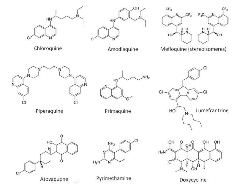
The use of topological descriptors is the key method, regardless of great advances taking place in the field of drug design. Descriptors portray the chemical characteristic of a molecule in numerical form, that is used for QSAR/QSPR models. The numerical values related with chemical constitutions that correlate the chemical structure with the physical properties refer to topological indices. The study of chemical structure with chemical reactivity or biological activity is termed quantitative structure activity relationship, in which topological index plays a significant role. Chemical graph theory is one such significant branch of science which plays a key role in QSAR/QSPR/QSTR studies. This work is focused on computing various degree-based topological indices and regression model of nine anti-malaria drugs. Regression models are fitted for computed indices values with 6 physicochemical properties of the anti-malaria drugs are studied. Based on the results obtained, an analysis is carried out for various statistical parameters for which conclusions are drawn.
- degree-based topological indices,
- regression model,
- QSPR analysis
Citation: Xiujun Zhang, H. G. Govardhana Reddy, Arcot Usha, M. C. Shanmukha, Mohammad Reza Farahani, Mehdi Alaeiyan. A study on anti-malaria drugs using degree-based topological indices through QSPR analysis[J]. Mathematical Biosciences and Engineering, 2023, 20(2): 3594-3609. doi: 10.3934/mbe.2023167

Related Papers:

Abstract

The use of topological descriptors is the key method, regardless of great advances taking place in the field of drug design. Descriptors portray the chemical characteristic of a molecule in numerical form, that is used for QSAR/QSPR models. The numerical values related with chemical constitutions that correlate the chemical structure with the physical properties refer to topological indices. The study of chemical structure with chemical reactivity or biological activity is termed quantitative structure activity relationship, in which topological index plays a significant role. Chemical graph theory is one such significant branch of science which plays a key role in QSAR/QSPR/QSTR studies. This work is focused on computing various degree-based topological indices and regression model of nine anti-malaria drugs. Regression models are fitted for computed indices values with 6 physicochemical properties of the anti-malaria drugs are studied. Based on the results obtained, an analysis is carried out for various statistical parameters for which conclusions are drawn.

References

[1]	J. B. Liu, M. Arockiaraj, M. Arulperumjothi, S. Prabhu, Distance based and bond assitive topological indices of certain repurposed antiviral drug compounds tested for trating COVID-19, Int. J. Quantum Chem., 121 (2021), e26617. https://doi.org/10.1002/qua.26617 doi: 10.1002/qua.26617
[2]	N. Makoah, G. Pradel, Antimalarial drugs resistance in Plasmodium falciparum and the current strategies to overcome them, Microb. Pathog. Strategies Combating Sci. Technol. Edu., 1 (2013), 269–282.
[3]	A. Rauf, M. Naeem, A. Aslam, Quantitative structure-property relationship of edge weighted and degree- based entropy of benzene derivatives, Int. J. Quantum Chem., 122 (2022), e26839. https://doi.org/10.1002/qua.26839. doi: 10.1002/qua.26839
[4]	H. Ali, U. Babar, S. H. Arshad, A. Sajjad, On some neighbourhood degree-based indices of graphs derived from honeycomb structure, Konuralp J. Math., 9 (2021), 164–175.
[5]	K. Roy, Topological descriptors in drug design and modeling studies, Mol. Diversity, 8 (2004), 321–323. https://doi.org/10.1023/b:modi.0000047519.35591.b7 doi: 10.1023/b:modi.0000047519.35591.b7
[6]	J. M. Sigarreta, Extremal problems on exponential vertex-degree-based topological indices, Math. Biosci. Eng., 19 (2022), 6985–6995. https://doi.rog/10.3934/mbe.2022329 doi: 10.3934/mbe.2022329
[7]	J. M. Sigarreta, Mathematical properties of variable topological indices, Symmetry, 13 (2021), 43. https://doi.org/10.3390/sym13010043 doi: 10.3390/sym13010043
[8]	W. Gao, W. Wang, M. R. Farahani, Topological indices study of molecular structure in anticancer drugs, J. Chem., 2016 (2016), 3216327. https://doi.org/10.1155/2016/3216327 doi: 10.1155/2016/3216327
[9]	J. F. Zhong, A. Rauf, M. Naeem, J. Rahman, A. Aslam, Quantitative structure-property relationships (QSPR) of valency based topological indices with Covid-19 drugs and application, Arab. J. Chem., 14 (2021), 1–16. https://doi.org/10.1016/j.arabjc.2021.103240 doi: 10.1016/j.arabjc.2021.103240
[10]	S. A. K. Kirmani, P. Ali, F. Azam, Topological indices and QSPR/QSAR analysis of some antiviral drugs being investigated for the treatment of COVID-19 patients, Int. J. Quantum Chem., 121 (2021), 1–22. https://doi.org/10.1002/qua.26594 doi: 10.1002/qua.26594
[11]	M. C. Shanmukha, A. Usha, N. S. Basavarajappa, K. C. Shilpa, Graph entropies of porous graphene using topological indices, Comput. Theor. Chem., 1197 (2021), 1–11. https://doi.org/10.1016/j.comptc.2021.113142 doi: 10.1016/j.comptc.2021.113142
[12]	M. C. Shanmukha, A. Usha, K. C. Shilpa, N. S. Basavarajappa, M-polynomial and neighborhood M- polynomial methods for topological indices of porous graphene, Eur. Phys. J. Plus, 136 (2021), 1–16. https://doi.org/10.1140/epjp/s13360-021-02074-8. doi: 10.1140/epjp/s13360-021-02074-8
[13]	M. Randic, Comparative structure-property studies: Regressions using a single descriptor, Croat. Chem. Acta, 66 (1993), 289–312.
[14]	M. Randic, Quantitative structure-propert relationship: Boiling points and planar benzenoids, New J. Chem., 20 (1996), 1001–1009.
[15]	M. C. Shanmukha, N. S. Basavarajappa, K. C. Shilpa, A. Usha, Degree-based topological indices on anticancer drugs with QSPR analysis, Heliyon, 6 (2020), e04235. https://doi.org/10.1016/j.heliyon.2020.e04235 doi: 10.1016/j.heliyon.2020.e04235
[16]	W. Gao, M. R. Farahani, S. Wang, M. N. Husin, On the edge-version atom-bond connectivity and geometric arithmetic indices of certain graph operations, Appl. Math. Comput., 308 (2017), 11–17. https://doi.org/10.1016/j.amc.2017.02.046 doi: 10.1016/j.amc.2017.02.046
[17]	H. Wang, J. B. Liu, S. Wang, W. Gao, S. Akhter, M. Imran, M. R. Farahani. Sharp bounds for the general sum-connectivity indices of transformation graphs, Discrete Dyn. Nat. Soc., 2017 (2017), 2941615. https://doi.org/10.1155/2017/2941615 doi: 10.1155/2017/2941615
[18]	W. Gao, M. K. Jamil, A. Javed, M. R. Farahani, M. Imran, Inverse sum indeg index of the line graphs of subdivision graphs of some chemical structures, UPB Sci. Bull. B, 80 (2018), 97–104.
[19]	S. Akhter, M. Imran, W. Gao, M. R. Farahani, On topological indices of honeycomb networks and graphene networks, Hacettepe J. Math. Stat., 47 (2018), 19–35.
[20]	X. Zhang, X. Wu, S. Akhter, M. K. Jamil, J. B. Liu, M. R. Farahani, Edge-version atom-bond connectivity and geometric arithmetic indices of generalized bridge molecular graphs, Symmetry, 10 (2018), 751. https://doi.org/10.3390/sym10120751 doi: 10.3390/sym10120751
[21]	H. Yang, A. Q. Baig, W. Khalid, M. R. Farahani, X. Zhang, M-polynomial and topological indices of benzene ring embedded in P-type surface network, J. Chem., 2019 (2019), 7297253. https://doi.org/10.1155/2019/7297253 doi: 10.1155/2019/7297253
[22]	D. Y. Shin, S. Hussain, F. Afzal, C. Park, D. Afzal, M. R. Farahani, Closed formulas for some new degree based topological descriptors using Mpolynomial and boron triangular nanotube, Front. Chem., 8 (2021), 613873. https://doi.org/10.3389/fchem.2020.613873 doi: 10.3389/fchem.2020.613873
[23]	M. Cancan, S. Ediz, M. R. Farahani, On ve-degree atom-bond connectivity, sum-connectivity, geometric-arithmetic and harmonic indices of copper oxide, Eurasian Chem. Commun., 2 (2020), 641–645. https://doi.org/10.33945/SAMI/ECC.2020.5.11 doi: 10.33945/SAMI/ECC.2020.5.11
[24]	S. Ediz, M. Cancan, M. Alaeiyan, M. R. Farahani, Ve-degree and Ev-degree topological analysis of some anticancer drugs, Eurasian Chem. Commun., 2 (2020), 834–840. https://doi.org/10.22034/ECC.2020.107867 doi: 10.22034/ECC.2020.107867
[25]	S. Ediz, M. Alaeiyan, M. R. Farahani, M. Cancan, On Van, r and s topological properties of the Sierpinski triangle networks, Eurasian Chem. Commun., 2 (2020), 819–826. https://doi.org/10.33945/SAMI/ECC.2020.7.9 doi: 10.33945/SAMI/ECC.2020.7.9
[26]	F. Harary, Graph Theory, Addison-Wesely, Reading Mass, 1969. https://doi.org/10.21236/AD0705364
[27]	V. R. Kulli, College Graph Theory, Vishwa International Publications, Gulbarga, India, 2012.
[28]	I. Gutman, O. E. Polansky, Mathematical Concepts in Organic Chemistry, Springer, Berlin, 1986. https://doi.org/10.1515/9783112570180
[29]	S. Fajtlowicz, On Conjectures of Grafitti Ⅱ, Cong. Numer., 60 (1987), 189–197.
[30]	B. Furtula, I. Gutman, A forgotton topological index, J. Math. Chem., 53 (2015), 213–220. https://doi.org/10.1007/s10910-015-0480-z doi: 10.1007/s10910-015-0480-z
[31]	W. Zhao, M. C. Shanmukha, A. Usha, M. R. Farahani, K. C. Shilpa, Computing SS index of certain dendrimers, J. Math., 2021 (2021), 7483508. https://doi.org/10.1155/2021/7483508. doi: 10.1155/2021/7483508
[32]	P. S. Ranjini, V. Lokesha, A. Usha, Relation between phenylene and hexagonal squeeze using harmonic index, Int. J. Graph Theory, 1 (2013), 116–121.

Reader Comments

Your name:*

Email:*
© 2023 the Author(s), licensee AIMS Press. This is an open access article distributed under the terms of the Creative Commons Attribution License (http://creativecommons.org/licenses/by/4.0)