Deep arrhythmia classification based on SENet and lightweight context transform

Yuni Zeng; Hang Lv; Mingfeng Jiang; Jucheng Zhang; Ling Xia; Yaming Wang; Zhikang Wang; Yuni Zeng; Hang Lv; Mingfeng Jiang; Jucheng Zhang; Ling Xia; Yaming Wang; Zhikang Wang

doi:10.3934/mbe.2023001

Mathematical Biosciences and Engineering

2023, Volume 20, Issue 1: 1-17. doi: 10.3934/mbe.2023001

Previous Article Next Article

Theory article Special Issues

Deep arrhythmia classification based on SENet and lightweight context transform

1.
School of Information Science and Technology, Zhejiang Sci-Tech University, Hangzhou 310018, China
2.
Department of Clinical Engineering, The Second Affiliated Hospital, School of Medicine, Zhejiang University, Hangzhou 310019, China
3.
Department of Biomedical Engineering, Zhejiang University, Hangzhou 310027, China
4.
Lishui University, Lishui 323000, China

Received: 15 July 2022 Revised: 04 September 2022 Accepted: 12 September 2022 Published: 29 September 2022

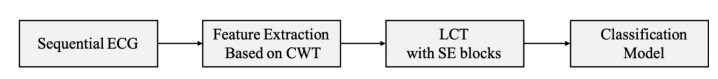
Arrhythmia is one of the common cardiovascular diseases. Nowadays, many methods identify arrhythmias from electrocardiograms (ECGs) by computer-aided systems. However, computer-aided systems could not identify arrhythmias effectively due to various the morphological change of abnormal ECG data. This paper proposes a deep method to classify ECG samples. Firstly, ECG features are extracted through continuous wavelet transform. Then, our method realizes the arrhythmia classification based on the new lightweight context transform blocks. The block is proposed by improving the linear content transform block by squeeze-and-excitation network and linear transformation. Finally, the proposed method is validated on the MIT-BIH arrhythmia database. The experimental results show that the proposed method can achieve a high accuracy on arrhythmia classification.
- continuous wavelet transform,
- Squeeze-and-Excitation network,
- lightweight context transform,
- arrhythmia classification
Citation: Yuni Zeng, Hang Lv, Mingfeng Jiang, Jucheng Zhang, Ling Xia, Yaming Wang, Zhikang Wang. Deep arrhythmia classification based on SENet and lightweight context transform[J]. Mathematical Biosciences and Engineering, 2023, 20(1): 1-17. doi: 10.3934/mbe.2023001

Related Papers:

Abstract

Arrhythmia is one of the common cardiovascular diseases. Nowadays, many methods identify arrhythmias from electrocardiograms (ECGs) by computer-aided systems. However, computer-aided systems could not identify arrhythmias effectively due to various the morphological change of abnormal ECG data. This paper proposes a deep method to classify ECG samples. Firstly, ECG features are extracted through continuous wavelet transform. Then, our method realizes the arrhythmia classification based on the new lightweight context transform blocks. The block is proposed by improving the linear content transform block by squeeze-and-excitation network and linear transformation. Finally, the proposed method is validated on the MIT-BIH arrhythmia database. The experimental results show that the proposed method can achieve a high accuracy on arrhythmia classification.

References

[1]	H. Chen, L. Shi, M. Xue, N. Wang, X. Dong, Y. Cai, et al., Geographic variations in in-hospital mortality and use of percutaneous coronary intervention following acute myocardial infarction in China: A nationwide cross-sectional analysis, J. Am. Heart Assoc., 7 (2018), e008131. https://doi.org/10.1161/JAHA.117.008131 doi: 10.1161/JAHA.117.008131
[2]	S. Yang, H. Shen, Heartbeat classification using discrete wavelet transform and kernel principal component analysis, in IEEE 2013 Tencon-Spring., Sydney, Australia, (2013), 34–38. https://doi.org/10.1109/TENCONSpring.2013.6584412
[3]	J. Park, S. M. Hwang, J. W. Baek, Y. N. Kim, J. H. Lee, Cardiac arrhythmias auto detection in an electrocardiogram using computer-aided diagnosis algorithm, in Applied Mechanics and Materials., (2014), 2728–2731. https://doi.org/10.4028/www.scientific.net/AMM.556-562.2728
[4]	T. Xia, M. Shu, H. Fan, L. Ma, Y. Sun, The development and trend of ECG diagnosis assisted by artificial intelligence, in Proceedings of the 2019 2nd International Conference on Signal Processing and Machine Learning, ACM, New York, USA, (2019), 103–107. https://doi.org/10.1145/3372806.3372807
[5]	S. Kaplan Berkaya, A. K. Uysal, E. S. Gunal, S. Ergin, S. Gunal, M. B. Gulmezoglu, A survey on ECG analysis, Biomed. Signal Process. Control, 43 (2018), 216–235. https://doi.org/10.1016/j.bspc.2018.03.003 doi: 10.1016/j.bspc.2018.03.003
[6]	A. Çınar, S. A. Tuncer, Classification of normal sinus rhythm, abnormal arrhythmia and congestive heart failure ECG signals using LSTM and hybrid CNN-SVM deep neural networks, Comput. Methods Biomech. Biomed. Eng., 24 (2021), 203–214. https://doi.org/10.1080/10255842.2020.1821192 doi: 10.1080/10255842.2020.1821192
[7]	Z. Wang, H. Li, C. Han, S. Wang, L. Shi, Arrhythmia classification based on multiple features fusion and random forest using ECG, J. Med. Imaging Health Inf., 9 (2019), 1645–1654. https://doi.org/10.1166/jmihi.2019.2798 doi: 10.1166/jmihi.2019.2798
[8]	S. Sabut, O. Pandey, B. S. P. Mishra, M. Mohanty, Detection of ventricular arrhythmia using hybrid time–frequency-based features and deep neural network, Phys. Eng. Sci. Med., 44 (2021), 135–145. https://doi.org/10.1007/s13246-020-00964-2 doi: 10.1007/s13246-020-00964-2
[9]	H. Zhang, K. Dana, J. Shi, Z. Zhang, X. Wang, A. Tyagi, et al., Context encoding for semantic segmentation, in 2018 IEEE/CVF Conference on Computer Vision and Pattern Recognition, Salt Lake City, USA, (2018), 7151–7160. https://doi.org/10.1109/CVPR.2018.00747
[10]	K. Xu, J. Ba, R. Kiros, K. Cho, A. Couville, R. Salakhutdinov, et al., Show, attend and tell: Neural image caption generation with visual attention, in International Conference on Machine Learning, PMLR, (2015), 2048–2057.
[11]	J. Hu, L. Shen, G. Sun, Squeeze-and-excitation networks, in IEEE Transactions on Pattern Analysis and Machine Intelligence, IEEE, 42 (2018), 7132–7141. https://doi.org/10.1109/TPAMI.2019.2913372
[12]	X. Chu, B. Zhang, R. Xu, MoGA: Searching beyond mobilenetv3, in 2020 IEEE International Conference on Acoustics, Speech and Signal Processing (ICASSP), IEEE, Barcelona, Spain (2020), 4042–4046. https://doi.org/10.1109/ICASSP40776.2020.9054428
[13]	D. Ruan, J. Wen, N. Zheng, M. Zheng, Linear context transform block, in Proceedings of the AAAI Conference on Artificial Intelligence, AAAI, New York, USA 34 (2020), 5553–5560. https://doi.org/10.1609/aaai.v34i04.6007
[14]	M. S. Moustafa, S. A. Sayed, Satellite imagery super-resolution using squeeze-and-excitation-based GAN, Int. J. Aeronaut. Space Sci., 22 (2021), 1481–1492. https://doi.org/10.1007/s42405-021-00396-6 doi: 10.1007/s42405-021-00396-6
[15]	S. Woo, J. Park, J. Y. Lee, I. S. Kweon, CBAM: Convolutional block attention module, in Proceedings of the European conference on computer vision (ECCV), (2018), 3–19. https://doi.org/10.1007/978-3-030-01234-2_1
[16]	M. F. Guo, X. D. Zeng, D. Y. Chen, N. C. Yang, Deep-learning-based earth fault detection using continuous wavelet transform and convolutional neural network in resonant grounding distribution systems, IEEE Sens. J., 18 (2017), 1291–1300. https://doi.org/10.1109/JSEN.2017.2776238 doi: 10.1109/JSEN.2017.2776238
[17]	Z. Wu, T. Lan, C. Yang, Z. Nie, A novel method to detect multiple arrhythmias based on time-frequency analysis and convolutional neural networks, IEEE Access, 7 (2019), 170820–170830. https://doi.org/10.1109/ACCESS.2019.2956050 doi: 10.1109/ACCESS.2019.2956050
[18]	T. Wang, C. Lu, Y. Sun, M. Yang, C. Liu, C. Ou, Automatic ECG classification using continuous wavelet transform and convolutional neural network, Entropy, 23 (2021), 119. https://doi.org/10.3390/e23010119 doi: 10.3390/e23010119
[19]	A. Ajit, K. Acharya, A. Samanta, A review of convolutional neural networks, in 2020 International Conference on Emerging Trends in Information Technology and Engineering (ic-ETITE), IEEE, Vellore, India, (2020), 1–5. https://doi.org/10.1109/ic-ETITE47903.2Vellore,India020.049
[20]	Y. Lu, M. Jiang, L. Wei, J. Zhang, Z. Wang, B. Wei, et al., Automated arrhythmia classification using depthwise separable convolutional neural network with focal loss, Biomed. Signal Process. Control, 69 (2021), 102843. https://doi.org/10.1016/j.bspc.2021.102843 doi: 10.1016/j.bspc.2021.102843
[21]	G. B. Moody, R. G. Mark, The impact of the MIT-BIH arrhythmia database, IEEE Eng. Med. Biol. Mag., 20 (2001), 45–50. https://doi.org/10.1109/51.932724 doi: 10.1109/51.932724
[22]	ANSI/AAMI EC57: 2012/(R)2020, Testing and reporting performance results of cardiac rhythm and ST segment measurement algorithms, 2012. Available from: https://array.aami.org/doi/10.2345/9781570204784.ch1
[23]	T. Mar, S. Zaunseder, J. P. Martínez, M. Llamedo, R. Poll, Optimization of ECG classification by means of feature election, IEEE Trans. Biomed. Eng., 58 (2011), 2168–2177. https://doi.org/10.1109/TBME.2011.2113395 doi: 10.1109/TBME.2011.2113395
[24]	V. Mondéjar-Guerra, J. Novo, J. Rouco, M. G. Penedo, M. Ortega, Heartbeat classification fusing temporal and morphological information of ECGs via ensemble of classifiers, Biomed. Signal Process. Control, 47 (2019), 41–48. https://doi.org/10.1016/j.bspc.2018.08.007 doi: 10.1016/j.bspc.2018.08.007
[25]	P. D. Chazal, M. O'Dwyer, R. B. Reilly, Automatic classification of heartbeats using ECG morphology and heartbeat interval features, IEEE Trans. Biomed. Eng., 51 (2004), 1196–1206. https://doi.org/10.1109/TBME.2004.827359 doi: 10.1109/TBME.2004.827359

Reader Comments

Your name:*

Email:*
© 2023 the Author(s), licensee AIMS Press. This is an open access article distributed under the terms of the Creative Commons Attribution License (http://creativecommons.org/licenses/by/4.0)